Podcast: Play in new window | Download | Embed
Episode Summary:
In this episode of Learning Machines 101, we review Chapter 6 of my book “Statistical Machine Learning” which introduces methods for analyzing the behavior of machine inference algorithms and machine learning algorithms as dynamical systems. We show that when dynamical systems can be viewed as special types of optimization algorithms, the behavior of those systems even when they are highly nonlinear and high-dimensional can be analyzed.
Show Notes:
Hello everyone! Welcome to the 84th podcast in the podcast series Learning Machines 101. In this series of podcasts my goal is to discuss important concepts of artificial intelligence and machine learning in hopefully an entertaining and educational manner.
This particular podcast is actually the seventh episode in a special series of episodes designed to provide commentary of my new book. The book’s title is “Statistical Machine Learning: A unified framework” published by CRC Press in their “Texts in Statistical Science” series. The basic idea of the book is that it is designed to provide mathematical tools from the fields of nonlinear optimization theory and mathematical statistics for the analysis and design of machine learning algorithms. If you have an undergraduate degree in computer science or engineering or math, then this book is a great way to get up-to-speed with some of the most important widely used mathematical tools in machine learning used by the top experts in machine learning. You can learn more about my new book by visiting the website: www.statisticalmachinelearning.com.
Each podcast in this special series describes a chapter from my new book. Each podcast is typically divided into four sections. The first section provides an easy-to-understand self-contained overview of the key concepts from the relevant chapter. The second section is specifically designed to provide guidance to the human student who is using the book for self-study. The third section is designed to provide guidance for the human instructor who is using the book for instruction. The fourth section is designed to provide guidance for robot web spiders (also called web spiderbots or web crawlers) so they can find this podcast and properly index it for humans. But even if you are not a robot web spider…you shouldn’t feel left out! Humans familiar with the relevant terminology will also find this fourth section of the podcast useful for a quick technical overview of what is covered in the book chapter.
The main focus of this particular episode covers the material in Chapter 6 of my new forthcoming book titled “Statistical Machine Learning: A unified framework.” Chapter 6 is titled “Convergence of Time-Invariant Dynamical Systems”.
[MUSICAL INTERLUDE]
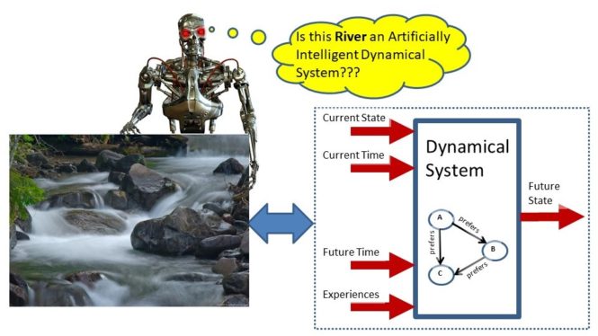
Before one can analyze a machine learning algorithm, the machine learning algorithm must be formally defined. Dynamical systems theory provides a formal framework for specifying and defining machines. Dynamic systems have properties which can change in time. At any particular instant in time, all properties relevant to specifying the exact behavior of the dynamical system can be specified as a list of numbers or equivalently a vector of numbers called the “system state vector”. The system state vector is a point in a high-dimensional space called the “system state space”. A dynamical system is simply a function which maps a point in a system state space at the current instant in time into another point in system state space at some future instant in time. So the basic idea is that a physical machine can be represented as a function which specifies how the current inputs, internal states, history of inputs, and outputs of the machine at the current instant in time determine the machine’s internal states and outputs at a future instant in time.
This function is called a dynamical system model of the machine. In real life, physical machines have certain intrinsic properties so we also introduce some additional constraints on the dynamical system. This discussion can be found in a recently released previous podcast: Learning Machines 101 Podcast Number 81 How to Define Machine Learning (at least try). In addition, we are interested in “smart machines” and Podcast 81 introduces one idea for defining the concept of “smart” for a dynamical system machine. The basic idea is that we view the dynamical system machine as transforming the current system state at the current instant in time into a “better” new system state at some future instant in time in such a way that we would consider the machine’s behavior to be “smart”. More formally, we have a function called the “risk function” which maps a system state into a number. The current system state is “preferred” to a future system state if the risk function evaluated at the future system state has a smaller value than the risk function evaluated at the current system state. We can use the concept of a “risk function” to help us analyze the behavior of highly complicated nonlinear high-dimensional dynamical system machines.
The Mississippi River is a river in the United Stated. Suppose we want to cross the Mississippi River in a row boat and we are in a portion of the river where the water currents are swirling around in vortices or whirlpools and we could get sucked into one of these whirlpool vortices and quickly perish. In this portion of the river, there are about 100 billion water molecules which is roughly equal to the number of neurons in the neocortical region of the human brain. One approach for deciding how to cross the river would be to write down a mathematical equation for the behavior of each of the 100 billion water molecules to describe how it moves in three-dimensional space. The current position of the 100 billion water molecules would be a point in the system state space. The dynamics of the river are specified by a dynamical system which maps one point in the system state space into another point in the system state space. The dynamical system is specified by 100 billion interacting nonlinear equations which describe the physical motion of the 100 billion water molecules in the river.
This is the type of problem faced by someone who is in the area of machine learning who wants to analyze or design a nonlinear learning machine or neural network learning algorithm which might have nonlinear dynamics of comparable complexity.
Although the actual solution of the 100 billion equations is computationally impossible, there is an approach which provides important insights into the dynamics. Lyapunov function methods work by showing that it is possible to identify the vortices or whirlpools in the river by studying the structure of the Lyapunov function rather than the original high-dimensional dynamical system. This is only possible because the dynamics of the high-dimensional dynamical system are implicitly linked to the Lyapunov function through the constraint that the Lyapunov function’s value never increases on trajectories generated by the dynamical system.
This is only a partial and limited analysis but it could provide a lot of insights into the river dynamics and also help provide us guidance regarding how to cross the river by avoiding river vortices. That is, we often are satisfied with characterizing general features of such systems because exact analyses of such systems are not available.
Let’s now consider a few representative Machine Learning examples which are covered in Chapter 6.
For our first example, consider a batch learning process where the goal of learning for a learning machine is to update its parameters based upon a particular training data set. Typically, one provides the learning machine with an initial random guess for the parameter values. Then the parameters of the learning machine are updated using all of the training data which are designed to result in improved estimates of the parameter values. This process is then iteratively repeated. The parameter values of the learning machine at any given point in time are referred to as a system state vector. The set of all possible values of the system state vector is called the system state space. A particular element of the system state vector is called a system state variable so here a particular parameter of the learning machine corresponds to a system state variable. The learning machine dynamical system is a function which maps the current system state vector at the current time point into a new system state vector at some future time point. Our goal is to try to design this function so that each time we apply this transformation we obtain a better set of parameter values for the learning machine.
Not that in batch learning, updates can be done in discrete-time or continuous-time. A discrete-time update assumes that time is discretized and the learning process which updates the parameter values occurs in different slices of times. Essentially any digital computer implementation of a batch learning algorithm is a discrete-time learning process. However, when developing specialized analog computers such as biological computers or parallel hardware machines or in contexts where information is naturally processed and represented in continuous time such as “speech data” or “robot motor control data” it may be important to investigate the behavior of continuous-time batch learning machines. Chapter 6 provides an introduction to mathematical tools for analyzing the behaviors of both discrete-time and continuous-time batch learning algorithms.
For our second example, a learning machine which already has a knowledge base but must make inferences based upon its knowledge. In this setup, the system state vector might consist of a collection of binary variables which specify whether a particular assertion about the world is either “true” or “false”. Specifically, a particular assertion corresponds to a particular binary state variable in the state vector which takes on the value of “1” when that assertion is true and takes on the value of “0” when that assertion is false. Some of the binary state variables have values which are known or “clamped” while the remaining binary state variables have values which are unknown or “unclamped”. The learning machine generates inferences about the world by mapping the current binary state vector and knowledge base at the current instant in time into a new binary state vector at some future time point. Only the binary state variables which are unclamped are modified. Sometimes this iterative process can be completed in a single step but in other cases this iterative process must be repeated multiple times in order to obtain a reasonable set of inferences. We refer to the dynamical system which updates the binary state vector as an inference machine dynamical system.
A third example, of a dynamical system relevant to machine learning problems is a “clustering algorithm” which can be interpreted as a type of inference machine dynamical system. Here, one provides the learning machine with a collection of patterns. The learning machine’s job is to group the patterns into clusters. This is achieved by updating a system state vector with binary variables where the values of the binary variables indicate whether or not a particular pattern belongs to a particular cluster. The dynamical system moves patterns from one cluster to another during the inference process with the goal of eventually obtaining a useful way of grouping the pattern vectors. That is, the dynamical system maps one grouping of the pattern vectors into a new grouping of the pattern vectors.
Ok…so now that we have some idea regarding examples of dynamical systems, how can we approach the problem of analyzing the behavior of such systems? Typically, such systems are highly nonlinear and have a high dimensionality so it would seem very difficult to obtain any insights into the behavior of such systems aside from simulation studies. However, there are some useful analyses which can be important for both guiding and interpreting simulations of dynamical systems.
Previously we introduced the concept of a “risk function” which is used to specify the preference semantics for an inference or learning machine. Dynamical systems theory is not concerned with semantics but is mainly focused upon characterizing the behavior of machines. Nevertheless, a dynamical system which is minimizing a risk function in a special way can be analyzed using an approach in dynamical systems theory called the Lyapunov function dynamical system analysis approach.
Just like a risk function used to represent preferences for a dynamical system, a Lyapunov function maps a point in system state space into a number. Lyapunov functions, however, also have the critical property that each time the dynamical system transforms the current system state into a new system state, the Lyapunov function evaluated at the new system state will not be larger than the Lyapunov function evaluated at the current system state. So, like the risk function concept, the idea is to construct a Lyapunov function so that one can interpret the dynamical system as seeking a system state that minimizes the Lyapunov function’s value. Our goal is to try to investigate a dynamical system’s behavior which is generating a sequence of high-dimensional state vectors by evaluating the Lyapunov function at each of the state vectors in the sequence to obtain a sequence of numbers. Then we will study the sequence of numbers and attempt to make some deductions about the behavior of the original sequence of high-dimensional state vectors.
There are some important subtleties associated with this sort of analysis that we should discuss. We first consider the simplest case where the state space is finite. An example of a finite state space would be the set of all d-dimensional binary state vectors. An example of a state space is not finite would be a state space whose points correspond to particular learning machine parameter vectors. Since parameter vectors have elements which are real numbers, the number of possible parameter vectors is uncountably infinite.
If the state space is finite and we have a Lyapunov function, then notice that each time the dynamical system transforms the current system state to a new system state, the dynamical system can never transform a future system state back to the current system state. Since there are only a finite number of states, this means that all future system state vectors are now confined to a smaller region of the finite state space.
If the system state is transformed back to itself by the dynamical system and consequently remains in that state for all future time it is called an “equilibrium point”. Thus, all sequences of states generated by the dynamical system in this context converge to the set of system equilibrium points.
This is an important and profound observation. It basically is saying that we characterizing the behavior of a high-dimensional nonlinear dynamical system by mapping the evolution of the high dimensional system states into a sequence of numbers using the Lyapunov function concept. Then, we can say something about the behavior of the original time evolution of high-dimensional system states.
This only works, however, because the state space is finite. If the state space is not finite, then additional conditions can be introduced to ensure convergence. These additional conditions are discussed in Chapter 6 and carefully explained with examples. Here, we provide a very quick overview.
Briefly, if the dynamical system is a discrete-time dynamical system where time is represented as a collection of countably infinite points, then the Lyapunov function has to be continuous. This is one of the most important conditions that we need for a Lyapunov function when the state space is not finite. It is important because the definition of a “continuous function” states that a sufficiently small change in the input to a continuous function will result in a sufficiently small change in the function’s output. Since the input of the continuous Lyapunov function is a state vector and the output is the value of the Lyapunov function which is a number, it follows that the assumption that the Lyapunov function is continuous provides the crucial relationship which helps us understand how convergence of system state vectors is related to convergence of Lyapunov function values generated by evaluating the Lyapunov function at each member of that convergent sequence of system state vectors.
If the dynamical system is a continuous-time dynamical system which the iterative process allows for an uncountably infinite number of time points, then the derivative of the Lyapunov function must be continuous.
In addition, when the state space is not finite, we will also require that the current system state is a continuous function of its initial state. This condition is not difficult to check in practice for either discrete-time or continuous-time systems.
We also need to show that the system state space is closed which means that if we generate a sequence of system state vectors using our dynamical system that the limit of that system state vectors is always inside the system state space. This sounds sort of strange but a good analogy is to think of each system state vector as specifying a point in 3-dimensional space. Now suppose we have a basketball and the system state space is the interior of the basketball so every system state vector specifies a point in 3-dimensional space which is inside the basketball. One could see that it is possible that there could be a sequence of points which is inside the basketball which is approaching a point located on the outside of the basketball. So this is an example where the system state space is not closed. This problem can be resolved sometimes by just redefining the system state space. In this case, we redefine the system state space to include not only the interior of the basketball but the outside of the basketball as well! Here we assume the basketball boundary is equivalent to the outside of the basketball.
And finally, we need to assume the system state space is bounded which means that all sequences of system state vectors generated by our dynamical system are confined to some finite region of the state space. Using our basketball analogy, we require that the system state space should fit into a basketball but the good news is that the basketball can be as large as we like. For example, we can choose a basketball the size of the known universe and that will work fine. We just can’t choose a basketball of infinite size!
With these assumptions, one can show that all sequences of system state vectors generated by our dynamical system converge to the collection of points where the change in the Lyapunov function’s value is zero. In addition, because the function is a Lyapunov function, it follows that the dynamical system is transforming state vectors into “better state vectors” in the sense that they have smaller Lyapunov values.
So this is the essential idea of Chapter 6. Note that Chapter 6 only covers dynamical systems whose properties do not change in time. Thus, Chapter 6 can not handle learning machines where the learning rate or the updating algorithm changes as a function of time. Appropriate variations of the topics covered in Chapter 6 which correspond to important popular nonlinear optimization discrete-time algorithms will be covered in Chapter 7 (the next podcast). In addition, both Chapter 6 and Chapter 7 are concerned with the analysis of deterministic batch learning algorithms but do not provide mathematical tools for analyzing adaptive learning algorithms. Adaptive learning algorithm will be covered in a future podcast when we review Chapter 12.
[MUSICAL INTERLUDE]
This section of the podcast is designed to provide guidance for the student whose goal is to read Chapter 6. When you read Section 6.1 which discusses Dynamical System Existence Theorems spend a lot of time studying the discrete-time case and make sure you really understand it. You can skip the continuous-time case temporarily and come back to it later. Read sections 6.3.1 and 6.3.2 on Lyapunov convergence theorems carefully but feel free to skip Example 6.3.3 for now. In section 6.3.2.2, I would recommend that you start by studying Theorem 6.3.1 which discusses the finite state space case. Study the finite state space proof very carefully. This is a very short theorem with a very easy proof. This will eventually help you appreciate the nuances of the much more complicated situation where the state space is not finite. Then move on to Recipe Box 6.1 and compare the contents of Recipe Box 6.1 with the statement of Theorem 6.3.2.
Theorem 6.3.2 is the key theorem of the entire chapter. It provides a strategy for analyzing the asymptotic behavior of a large class of time-invariant discrete-time and continuous-time dynamical systems. The theorem is applicable to systems with multiple equilibrium points and does not require that the Lyapunov function is a convex function. The only requirements on the Lyapunov function are that it is sufficiently smooth and that it is non-increasing on the trajectories of the dynamical system.
Also work through Examples 6.3.5 and 6.3.6 carefully. Supplemental readings can be found at the end of the chapter. The textbook by Hirsch, Smale, and Devaney titled “Differential Equations, Dynamical Systems, and an Introduction to Chaos” published in 2013 by Academic Press is particularly recommended. This is a great textbook written at the level of my textbook for advanced undergraduate students or first year graduate students in engineering, math, or computer science.
[MUSICAL INTERLUDE]
This section of the podcast is designed to provide guidance to the instructor whose goal is to teach Chapter 6. Remember these notes are available for download by simply visiting this episode on the website: www.learningmachines101.com. In addition, supplemental teaching materials and errata for the book (as they become available) will be available on the website: www.statisticalmachinelearning.com.
I would begin this chapter by possibly reviewing selected material from Section 3.2 in which the concept of a dynamical system is introduced as a general purpose mathematical formalism for representing a “machine”. In introductory lower-division courses in differential equations and dynamical systems, the distinction between systems of differential and difference equations and dynamical systems is not often carefully emphasized and explained. So it is worth spending some time clarifying this distinction. Otherwise, the first section of the Chapter 6.1 which discusses existence and uniqueness theorems will not make any sense to students if they think that a system of differential equations is a dynamical system when, in fact, the solution of the system of differential equations provides the dynamical system specification.
After this is explained, it would be helpful to provide concrete examples of machine learning algorithms which will be analyzed in this chapter and describing them within a dynamical systems framework. You might want to consider discussing Example 3.2.1 and Exercise 6.1-4 (discrete-time gradient descent), Example 3.2.5, Exercise 6.1-3, and Exercise 6.1-5 (continuous-time gradient descent), and 6.3-7 (clustering algorithms).
For a standard machine learning course, you might want to skip Chapter 6 since many of the key ideas are covered in Chapter 7 using more classical nonlinear optimization algorithms. However, if the students are interested in continuous-time dynamical systems such as students interested in “speech recognition”, “robot control”, or computational neuroscience then this is a great chapter to include.
[MUSICAL INTERLUDE]
This section is designed mainly for search engines and web spider robots but humans will find this final section relevant also!!
The objective of Chapter 6 is to provide methods for providing sufficient conditions for ensuring that time-invariant discrete-time and time-invariant continuous-time dynamical systems will converge to either an isolated critical point or a collection of critical points. Such dynamical systems are often used to represent inference algorithms and batch learning algorithms. The concept of a Lyapunov function is then introduced for analyzing the dynamics of discrete-time and continuous-time dynamical systems. A Lyapunov function tends to decrease as the dynamical system evolves. It is not assumed that the Lyapunov function is a convex function although stronger results (of course) will be obtained in such cases.
The Finite State Space Invariant Set Theorem (Theorem 6.3.1) is introduced for the purpose of proving the convergence of a discrete-time dynamical system on a finite state space. Next, an extension of LaSalle’s (1960) Invariant Set Theorem (Theorem 6.3.2) is introduced for providing sufficient conditions for the trajectories of a discrete-time or continuous-time dynamical system to converge to either an individual critical point or a collection of critical points. These convergence theorems are then used to investigate the asymptotic behavior of commonly used batch learning algorithms such as: gradient descent, and ADAGRAD. These convergence theorems are also used to investigate the asymptotic behavior of clustering algorithms, the ICM (iterated conditional modes) algorithm, the Hopfield (1982) algorithm, and the BSB (Brain-State-in-a-Box) algorithm.
[MUSICAL INTERLUDE]
My new book “Statistical Machine Learning” can be purchased right now at an 18% discount for the hard copy which is about $98 and a 64% discount for the Kindle version so the Kindle version is $43.41. You can purchase the book by going to AMAZON.com or you can go to the CRC publisher website which is easily accessed by visiting: www.statisticalmachinelearning.com.
I apologize for the irregular podcast production in the year 2020. Hopefully, in the year 2021 I will be able to have a more regular podcast production schedule. My goal is to generate a new podcast once a month during the 2021 year which will effectively provide a broad overview of my new book. Entirely new podcasts are being planned for future years beyond 2021 as well!!!
So make sure to subscribe to my podcast Learning Machines 101: A Gentle Introduction to Artificial Intelligence and Machine Learning on Apple Podcast, STITCHER, GOOGLE podcast, or your favorite podcast service provider!! Also join the Learning Machines 101 community and let me know your ideas for future podcasts!!!
If you are not a member of the Learning Machines 101 community, you can join the community by visiting our website at: www.learningmachines101.com and you will have the opportunity to update your user profile at that time. This will allow me to keep in touch with you and keep you posted on the release of new podcasts and book discounts. You can update your user profile when you receive the email newsletter by simply clicking on the: “Let us know what you want to hear” link!
In addition, I encourage you to join the Statistical Machine Learning Forum on LINKED-IN. When the book is available, I will be posting information about the book as well as information about book discounts in that forum as well.
And don’t forget to follow us on TWITTER. The twitter handle for Learning Machines 101 is “lm101talk”! Also please visit us on Apple Podcast or Stitcher and leave a review. You can do this by going to the website: www.learningmachines101.com and then clicking on the Apple Podcast or Google Podcast or Stitcher.com. This will be very helpful to this podcast! Thank you again so much for listening to this podcast and participating as a member of the Learning Machines 101 community!
And finally…please take care of yourselves and your neighbors in this difficult time by practicing social distancing. In fact, if you want to make a donation to the World Health Organization, you can find a hyperlink to help you do this on the main page of the learning machines 101 website.
Take Care and See you soon!!
REFERENCES:
Golden, R. M. (2020). Statistical Machine Learning: A Unified Framework.
CRC Press. (Chapter 6). [Good introduction for undergraduate and graduate students.]
LaSalle, J. (1960). Some extensions of Liapunov’s second method. IRE Transactions on Circuit Theory, 7, 520-527. [Advanced but classic article!]
Related Learning Machines 101 Podcasts:
Episode LM101-081: Ch3: How to Define Machine Learning (or at Least Try)
