Podcast: Play in new window | Download | Embed
Episode Summary:
This particular podcast covers the material in Chapter 4 of my new book “Statistical Machine Learning: A unified framework” which is now available! Many important and widely used machine learning algorithms may be interpreted as linear machines and this chapter shows how to use linear algebra to analyze and design such machines. In addition, these same techniques are fundamentally important for the development of techniques for the analysis and design of nonlinear machines.
Show Notes:
Hello everyone! Welcome to the 82nd podcast in the podcast series Learning Machines 101. In this series of podcasts my goal is to discuss important concepts of artificial intelligence and machine learning in hopefully an entertaining and educational manner.
This particular podcast is actually the fourth episode in a special series of episodes designed to provide commentary of my new book. The book’s title is “Statistical Machine Learning: A unified framework” published by CRC Press in their “Texts in Statistical Science” series. The basic idea of the book is that it is designed to provide mathematical tools from the fields of nonlinear optimization theory and mathematical statistics for the analysis and design of machine learning algorithms. If you have an undergraduate degree in computer science or engineering or math, then this book is a great way to get up-to-speed with some of the most important widely used mathematical tools in machine learning used by the top experts in machine learning. You can learn more about my new book by visiting the website: www.statisticalmachinelearning.com.
Each podcast in this special series describes a chapter from my new book. Each podcast is typically divided into four sections. The first section provides an easy-to-understand self-contained overview of the key concepts from the relevant chapter. The second section is specifically designed to provide guidance to the human student who is using the book for self-study. The third section is designed to provide guidance for the human instructor who is using the book for instruction. The fourth section is designed to provide guidance for robot web spiders (also called web spiderbots or web crawlers) so they can find this podcast and properly index it for humans. But even if you are not a robot web spider…you shouldn’t feel left out! Humans familiar with the relevant terminology will also find this fourth section of the podcast useful for a quick technical overview of what is covered in the book chapter.
The main focus of this particular episode covers the material in Chapter 4 of my new forthcoming book titled “Statistical Machine Learning: A unified framework.” Chapter 4 is titled “Linear Algebra for Machine Learning”.
[music interlude]
There are many examples in machine learning where the common currency for communicating information is not a single number but a list of numbers. A list of numbers is called a “vector”.
For example, the concept of using a feature vector which is essentially a list of numbers was introduced and discussed in Episode 80 and Episode 81 of Learning Machines 101. Briefly, a feature vector represents information. One way to think of a feature vector is a list of numbers where the first number on the list specifies the activity level or response level or state of a simple processing unit. The second number in the feature vector specifies the state of the second processing unit. The third element of the feature vector specifies the state of the third processing unit and so on. If we assume there are 1000 processing units, then the feature vector is called a 1000-dimensional feature vector.
Another example is a parameter vector. The parameters of a learning machine are adjusted as the learning machine encounters experiences in its world. Assume the learning machine has 10,000 free parameters. Then each time the learning machine encounters a new experience in its environment which is typically represented as a feature vector, all 10,000 free parameters are slightly adjusted during the learning process. We can arrange all 10,000 free parameters as a long ordered list and this is what we call a parameter vector.
And so we see that the concept of a “vector” is actually fundamental to machine learning. It is a very convenient object for the purposes of representing and manipulating concepts and information. There is an entire mathematical theory designed for representing and manipulating vectors and this is called “linear algebra”. Just like you can add and subtract and multiply numbers, with “linear algebra” you can add and subtract and multiply vectors.
A really nice feature of vectors is their geometric interpretation. Suppose we have a learning machine which has only two parameters. Imagine a two-dimensional plot where the horizontal x-axis lists all possible values of the first parameter and the vertical y-axis list all possible values of the second parameter. A particular pair of parameter values for the learning machine would then be represented as just one point or dot in this two-dimensional plot.
After the learning machine has a learning experience, the parameters of the learning machine are adjusted slightly and this causes the point in this two-dimensional space to move by a slight amount. As the learning process continues, the parameters values of the learning machine continue to be adjusted. Geometrically, this means that the point now traces a curve through this two-dimensional space which represents the learning trajectory.
Now this same analysis actually works if we have a learning machine with three parameters instead of two parameters. In this case, we have a single point moving along a learning trajectory in a three-dimensional space. In fact, this analysis even works when the learning machine has 10,000 free parameters. In this case, we have a 10,000-dimensional space but the current parameter values of the learning machine are represented by a single point in this 10,000-dimensional space. So this is very nice because we can use our intuitions about geometry to begin to think about learning in high-dimensional spaces.
So, to summarize, the first important contribution of linear algebra is that it provides methods for looking at the similarity and differences between points in high-dimensional spaces. But that is not all.
Now consider a learning machine which has a numerical output. Assume the input to the learning machine is a 100-dimensional feature vector. In addition, assume the output of the learning machine is a weighted sum of the elements of the input feature vector where the
weights are free parameters. If the learning machine has 100 inputs, then it has 100 free parameters. Thus the output of the learning machine is computed using the following formula first input feature vector element multiplied by first parameter plus second input feature vector element multiplied by second parameter plus third input feature vector element multiplied by third parameter plus fourth input feature vector element multiplied by fourth parameter and so on.
Such a learning machine whose response is simply a weighted sum of its inputs is called a “Linear Machine”. A useful way of describing this computation involves the concept of a “dot product” operation. Briefly, the response of this linear machine may be concisely described as simply the dot product of the input vector with the linear machine’s parameter vector. If the dot product of the input vector with the linear machine’s parameter vector is zero, then by definition the linear machine’s output is equal to zero.
Geometrically, we can plot the parameter vector of the learning machine as a point in a high-dimensional state space. Then we can plot the input vector as a point in this same high-dimensional state space. Now we draw an arrow from the origin to the parameter vector point. We draw another arrow from the origin to the input vector point. It can be shown, interestingly enough, that the dot product between these two vectors is equal to the cosine of the angle between the two vectors multiplied by the length of the first vector and multiplied again by the length of the second vector. So the dot product operation can be viewed as an indirect way of measuring the similarity between two vectors by determining if they are pointing in the same direction.
So, to review, the output of a linear learning machine is simply the dot product of its input pattern vector with the parameter vector of the learning machine. The linear learning machine updates its parameter vector as it learns within its environment.
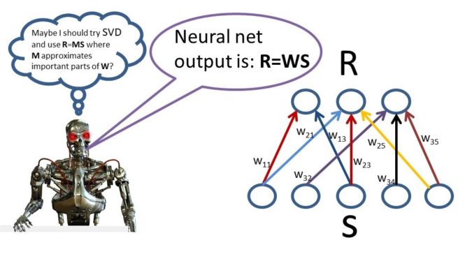
Let’s now define a processing unit whose output is defined as the dot product of an input pattern with its parameter vector. Now suppose that we have a collection of such processing units where each processing unit computes a dot product of its parameter vector with an input pattern vector. The pattern of activity generated by the collection of processing units will be called a response vector. Each element of the response vector is generated by computing the dot product of the parameter vector for the processing unit of that response vector with the input pattern. Now define an array of numbers whose first row is the parameter vector for the first processing unit. The second row is the parameter vector for the second processing unit. The third row is the parameter vector for the third processing unit and so on. This array of numbers is called a “matrix”. The number of rows in the matrix is equal to the number of processing units. The mathematical operation which generates the response vector given the matrix and the input vector is called a “matrix by vector” multiplication operation. So this is a nice high-level description of a fairly involved operation but this type of operation is highly used.
Compact representations such as “vectors” and “matrices” and compact operators such as “dot product” and “matrix multiplication” are extremely powerful because they allow us to visualize very complicated operations involving hundreds of thousands of linear processing units in terms of a few symbols. Not only is this useful from the perspective of understanding both linear and nonlinear learning machines, this is also useful for communicating in a terse and efficient way a series of complicated operations involving possibly millions of computing units operating in parallel. And furthermore, compact vector and matrix operations are also useful from the perspective of implementing such machines in software. Such mathematical operators can be and have been directly implemented as software functions and optimized to take advance of specialized parallel processing hardware such as GPUs.
Let’s now move to a discussion of knowledge representation interpretation in the linear machine. Consider the situation where we have a collection of processing units which transform an input Vector into a response vector using a matrix by vector multiplication operation. That is, the response vector is generated by multiplying the matrix of parameter values by the input vector. Intuitively, the parameter value in row I and column j of the matrix of parameter values indicates the degree to which the jth element in the input vector influences the ith element in the response vector.
This is a remarkably different way of thinking about knowledge representation. The knowledge representation specifies how the system responds to a particular input vector. This representation is not specified by a list of rules or symbolic look-up table. It is specified simply by a matrix of numbers. The first row of the matrix specifies the parameter vector of the first processing unit, the second row of the matrix specifies the parameter vector for the second processing unit, and so on.
So to summarize, suppose we have 10,000 input processing units. Each of the 10,000 processing units has a real-valued state so we can represent the state of activity over the 10,000 processing units as a list of 10,000 numbers or equivalently as a single symbol which is 10,000-dimensional vector. Now assume we have 5,000 output processing units where each output processing unit computes its state by computing a weighted sum of the states of the 10,000 input processing units. The state of activity over the 5,000 output processing units may be represented as a single symbol which is a 5,000-dimensional vector. In this system there are 5,000 multiplied by 10,000 free parameters or connection weights. These 50,000,000 connection weights are represented as an array of numbers with 5,000 rows and 10,000 columns or equivalently as a single symbol which is matrix. The 5,000 dimensional output vector state of this linear system is simply equal to the linear system’s matrix of 50,000,000 connection weights multiplied by an input vector with dimensionality 10,000. In software code, this operation would be represented using only five characters.
Often one has a collection of input pattern vectors and for each input pattern vector it is desired to generate a particular output pattern vector, a computationally useful method for analyzing the connection weight matrix which will generate the right output pattern vector for a given input pattern vector involves a concept called SVD or singular value decomposition.
Singular value decomposition methods can be very helpful for semantically interpreting or estimating the matrix of parameter values in a linear learning machine. The basic idea is that SVD provides a method for rewriting the matrix of parameter values learned by a linear learning machine as a “weighted sum” of matrices. For example, the original array of numbers might be rewritten as the number 100 multiplied by some other array of numbers which I will call Matrix 1 plus the number 10 multiplied by some other array of numbers which I will call Matrix 2 plus the number 0.0001 multiplied by some other array of numbers which I will call Matrix 3. The weighting factors 100, 10, and 0.0001 specify the degree to which each of these matrices contributes to the representation of the original matrix. Since the weight for Matrix 1 is 100 then the statistical regularities specified in Matrix 1 are very important but since the weight for Matrix 3 is 0.0001 then this means that the statistical regularities specified in Matrix 3 are likely to not be important but rather represent “statistical noise”. Thus, one might hypothesize that the important statistical regularities learned by the learning machine are NOT best represented by the actual parameter value matrix which was learned by rather by an approximation to the original matrix which is equal to Matrix 1 multiplied by 100 plus Matrix 2 multiplied by 10. The term in the weighted sum associated with Matrix 3 is eliminated because it is assumed that the information in Matrix 3 is noise.
So, in summary, rewriting a matrix as a weighted sum of other matrices provides a powerful tool for identifying important statistical regularities. The components of this weighted sum representing less relevant statistical regularities are weighted less strongly in the weighted sum of matrices than the matrices in the weighted sum representing important statistical regularities. Thus, in practice, unimportant and distracting statistical regularities extracted by the learning machine are often removed by deliberately omitting the matrices with the smaller weights from the weighted sum of matrices resulting in dramatic improvements in generalization performance.
SVD methods are very useful for providing simple formulas for setting the parameters of a linear learning machine so that it can recognize some feature vectors and ignore other feature vectors. So SVD methods can be used to design “instant learning algorithms” where you provide the learning machine with the input vectors and then in just one computation all of the parameter values of the learning machine are set to their correct values!!!
Many important machine learning algorithms are examples of linear learning machines or are closely related to linear learning machines. In addition, there are many more important machine learning algorithms which are not linear machines. A learning machine which is not a linear machine is called a nonlinear learning machine. Deep learning algorithms are examples of nonlinear learning machines. Still, it turns out that by obtaining a deep understanding of linear machines, this can not only help us understand linear learning machines but also provide essential steps towards developing mathematical tools for the analysis and design of nonlinear learning machines.
In many cases such analyses of nonlinear machines are possible by approximating such machines by linear machines in specific special situations. So, for example, if you have a highly complex nonlinear curve such a curve can be approximated by a series of short line segments. This essential idea lies at the heart of many important mathematical analyses of learning in highly nonlinear smooth systems as well as the study of generalization performance in nonlinear learning machines.
Thus, an understanding of linear machine analysis and design methods is an essential stepping stone to the analysis and design of nonlinear learning machines.
In the show notes of this episode, I have included some references to help you learn about linear algebra. There is a nice tutorial on linear algebra written by Michael Jordan in the mid-1980s designed for students with no formal knowledge of linear algebra. The show notes also include a link to the linear algebra course taught by Dr. Strang at MIT which is a free course. His linear algebra is a relatively easy lower-division introduction to linear algebra which covers the important points in a straightforward and easy to process manner. It is highly recommended as a first introduction to linear algebra and matrix operations. Finally, I have also included some advanced textbooks on linear algebra which contain material which are very useful in machine learning and mathematical statistics applications yet those topics are not typically covered in introductory lower-division linear algebra courses such as the course taught by Dr. Strang. So check out those references in the show notes of this episode at: www.learningmachines101.com.
[MUSICAL INTERLUDE]
This section of the podcast is designed to provide guidance for the student whose goal is to read Chapter 4. Although the material in Chapter 4 is self-contained, it is expected that the student has already completed a lower-division course in linear algebra. Most of the material in this Chapter will have been covered in such a lower-division linear algebra course. However, it is likely that the significance and importance of that material for machine learning was not explained or emphasized. Chapter 4 focuses on very selected aspects of linear algebra which are directly relevant to machine learning.
Make sure to study the notation and definitions in Section 4.1. In fact, you might want to take a look at Section 4.1 before you start reading Chapter 1 of the textbook.
Don’t spend much time on the Kronecker Matrix Product Identities but make a mental note that they are located in the book in case you need to reference them in the future. There will be material in Section 4.1 which will be new to you even if you have already taken linear algebra as an undergraduate. Sections 4.2 and 4.3 cover material which you should have encountered in your linear algebra class. Make sure you understand this material. However, the examples of how the linear algebra relates to machine learning will probably be brand new to you so study those carefully.
[MUSICAL INTERLUDE]
This section of the podcast is designed to provide guidance to the instructor whose goal is to teach Chapter 4. Remember these notes are available for download by simply visiting this episode on the website: www.learningmachines101.com. In addition, supplemental teaching materials (as they become available) will be available on the website: www.statisticalmachinelearning.com.
Chapter 4 is simply a review of relevant concepts from linear algebra which are especially important for machine learning. Although all students in the class have taken linear algebra, you will find that many of the students (if this is an advanced undergraduate or first year graduate course) will have forgotten important technical details and will find this review valuable. In addition, Section 4.1 includes useful matrix operators which might not be taught in the typical lower-division linear algebra class.
When teaching from my book, I cover the first few sections of Chapter 1 the first week of class but also require that all students in the class read Section 4.1 on their own. I don’t spend time in class reviewing matrix multiplication the first week of class but in the first week of class, I do introduce my matrix and vector notation which is boldface uppercase letters for matrices and lowercase boldface letters for vectors. In addition, I introduce special operators such as the Hadamard element by element matrix product operator, and the vec operator which stacks a matrix column by column into a vector, and vector-valued versions of commonly used operators such as natural logarithm.
After covering Chapter 1 and Section 4.1 in the first few weeks of class and then selected parts of Chapters 2 and 3, then after a few weeks the class will finally return to Chapter 4 and cover Sections 4.2 and 4.3. The focus of Sections 4.2 and 4.3 in Chapter 4 is on the use of singular value decomposition methods for matrix decomposition and solving systems of linear equations.
Finally, when teaching this material, it is highly recommended that you put more emphasis on the examples which illustrate how the linear algebra discussion supports machine learning applications. The students will learn the linear algebra more easily if they can see why it is so relevant and important for machine learning.
[MUSICAL INTERLUDE]
This section is designed mainly for search engines and web spider robots but humans will find this final section relevant also!!
The objective of Chapter 4 is to introduce advanced matrix operators and the singular value decomposition method for supporting the analysis and design of linear machine learning algorithms. More specifically, Chapter 4 begins with a review of basic matrix operations and definitions while introducing more advanced matrix operators for supporting the matrix calculus theory supported in Chapter 5. Definitions of the vec function, matrix multiplication, trace operator, Hadamard product, duplication matrix, positive definite matrices, matrix inverse, and matrix pseudoinverse are provided. The chapter also includes a collection of useful Kronecker matrix product identities to support advanced matrix calculus operations. In addition, Chapter 4 introduces singular value decomposition (SVD) as a tool for the analysis and design of machine learning algorithms. Applications of eigenvector analysis and singular value decomposition for latent semantic Indexing (LSI) and solving linear regression problems are provided. The chapter ends with a discussion of how the Sherman-Morrison Theorem may be applied to design adaptive learning algorithms that incorporate matrix inversion. In particular, the Sherman-Morrison Theorem provides a computational shortcut for recursively computing the inverse of a matrix generated from n+1 data points from the inverse of a matrix generated from n of the n+1 data points.
[MUSICAL INTERLUDE]
My new book “Statistical Machine Learning” can be purchased right now.
You can purchase the book at a 20% discount (but I don’t know how long this discount will last) on the CRC publisher’s website which can be reached by visiting the website: www.statisticalmachinelearning.com. Make sure to join the Learning Machines 101 community in order to be updated when and how book discounts will be available.
If you are not a member of the Learning Machines 101 community, you can join the community by visiting our website at: www.learningmachines101.com and you will have the opportunity to update your user profile at that time. This will allow me to keep in touch with you and keep you posted on the release of new podcasts and book discounts. You can update your user profile when you receive the email newsletter by simply clicking on the: “Let us know what you want to hear” link!
In addition, I encourage you to join the Statistical Machine Learning Forum on LINKED-IN. When the book is available, I will be posting information about the book as well as information about book discounts in that forum as well.
And don’t forget to follow us on TWITTER. The twitter handle for Learning Machines 101 is “lm101talk”! Also please visit us on Apple Podcast or Stitcher and leave a review. You can do this by going to the website: www.learningmachines101.com and then clicking on the Apple Podcast or Stitcher icon. This will be very helpful to this podcast! Thank you again so much for listening to this podcast and participating as a member of the Learning Machines 101 community!
And finally…please take care of yourselves and your neighbors in this difficult time by practicing social distancing. In fact, if you want to make a donation to the World Health Organization, you can find a hyperlink to help you do this on the main page of the learning machines 101 website.
Take Care and See you soon!!
REFERENCES:
Jordan, Michael (1986). An introduction to linear algebra for parallel distributed processing.
Book Chapter from PDP Book Series by Rumelhart, Hinton, and McClelland.
MIT online coursework also offers the FREE lower-division undergraduate linear algebra course “Linear Algebra” taught by Dr. Strang.
Strang, Gilbert. Introduction to Linear Algebra. 5th ed. Wellesley-Cambridge Press, 2016. ISBN: 9780980232776.
Schott, J. R. 2005. Matrix Analysis for Statistics (Second ed.). Wiley Series in Probability and Statistics. New Jersey: Wiley
Golden, R. M. (2020). Statistical Machine Learning: A Unified Framework.
CRC Press. (Chapter 4).
Franklin, J. N. (2000). Matrix Theory.
Banerjee, S. and A. Roy 2014. Linear Algebra and Matrix Analysis for Statistics. Texts in Statistical Science. Boca-Raton, FL: Chapman-Hall/CRC Press.
