Podcast: Play in new window | Download | Embed
Episode Summary:
This particular podcast covers the material in Chapter 3 of my new book “Statistical Machine Learning: A unified framework” with expected publication date May 2020. In this episode we discuss Chapter 3 of my new book which discusses how to formally define machine learning algorithms. Briefly, a learning machine is viewed as a dynamical system that is minimizing an objective function. In addition, the knowledge structure of the learning machine is interpreted as a preference relation graph which is implicitly specified by the objective function. In addition, this week we include in our book review section a new book titled “The Practioner’s Guide to Graph Data” by Denise Gosnell and Matthias Broecheler.
Show Notes:
Hello everyone! Welcome to the 81th podcast in the podcast series Learning Machines 101. In this series of podcasts my goal is to discuss important concepts of artificial intelligence and machine learning in hopefully an entertaining and educational manner.
This particular podcast is actually the third episode in a special series of episodes designed to provide commentary of my new forthcoming book. The book’s title is “Statistical Machine Learning: A unified framework” and it will be published by CRC Press in their “Texts in Statistical Science” series in May of this year 2020. The basic idea of the book is that it is designed to provide mathematical tools from the fields of nonlinear optimization theory and mathematical statistics for the analysis and design of machine learning algorithms. You can learn more about my new book by visiting the website: www.statisticalmachinelearning.com.
Each podcast in this special series describes a chapter from my new book. Each podcast is typically divided into four sections. The first section provides an easy-to-understand self-contained overview of the key concepts from the relevant chapter. The second section is specifically designed to provide guidance to the human student who is using the book for self-study. The third section is designed to provide guidance for the human instructor who is using the book for instruction. The fourth section is designed to provide guidance for robot web spiders (also called web spiderbots or web crawlers) so they can find this podcast and properly index it for humans. But even if you are not a robot web spider…you shouldn’t feel left out! Humans familiar with the relevant terminology will also find this fourth section of the podcast useful for a quick technical overview of what is covered in the book chapter.
Today, I also include an additional supplemental book review section on a new book titled “The Practitioner’s Guide to Graph Data” by Denise Gosnell and Matthias Broecheler which has just come out on the topic of “graph thinking” which I feel is a very important topic for researchers in machine learning.
The main focus of this particular episode, however, covers the material in Chapter 3 of my new forthcoming book titled “Statistical Machine Learning: A unified framework.” Chapter 3 is titled “Formal Machine Learning Algorithms”.
[music interlude]
Suppose that we were going to write a book about “Business Development”. Presumably, at the beginning of the book we would feel obligated to share with the reader our definition of a “Business Development”. As another example, if you pick up a book on “optimization theory”, then early on in the beginning of the book the author will define the generic optimization problem. If you pick up a book on “linear systems theory”, then early on in the beginning of the book the author will define the concept of a “linear system”. Still, many books on machine learning do not attempt to define in a formal manner what exactly is a machine learning algorithm.
Formal definitions have several purposes. First, without a formal definition of an assertion, then it is impossible to explore through deductive logic the implications of that assertion. Second, formal definitions are important for the purpose of communication. Suppose that I am trying to communicate to someone the concept of an “airplane”. I can tell them that an airplane is like a helicopter but the physics which makes the airplane fly is a little different. I can show them several examples of an airplane. But without a formal definition, it will be difficult to communicate exactly my understanding of an airplane to someone else. Third, formal definitions are important for the advancement of science. If I provide a formal definition of an airplane, then I have opened myself up for criticism. Other scientists and engineers can criticize my definition and suggest improvements. Without a formal definition, then it will be difficult to criticize that definition and the flaws in that definition are not revealed.
The problem of defining a “machine learning algorithm” is trickier than it sounds. One might start with the idea is that the definition of a machine learning algorithm is a “machine that learns from experience.” But this definition is almost circular.
What is the formal definition of a “machine”?
What is the formal definition of “learns”?
What is the formal definition of “experience”?
And so, in this spirt, I decided to write Chapter 3 of my new book which is about Machine Learning. My thinking was that if I’m writing a book about Machine Learning, I’m obligated (to at least try) to introduce a formal definition of Machine Learning. Accordingly, Chapter 3 represents a first attempt to formally define Machine Learning algorithms. Initially this Chapter was a lot longer and I chopped out many sections. In fact, at some point, I was playing with the idea of totally eliminating this Chapter but my students found it useful so I ended up keeping a relatively short version of the original Chapter. In any case, let’s begin!!!
Because the experiences of a learning machine influence its behavior, it is useful to develop a formal mathematical definition of the concept of an “experience”. An “environmental event” corresponds to a snapshot of the learning machine’s environment over a particular time period in a particular location. Examples of “events” include: the pattern of light rays reflecting off a photographic image, air pressure vibrations generated by a human voice, an imaginary situation, the sensory and physical experience associated with landing a lunar module on the moon, a document and its associated search terms, a consumer’s decision making choices on a website, and the behavior of the stock market.
In order to develop a mathematical model of a learning machine, it is necessary to develop a mathematical theory of the environment. Such a mathematical theory begins with the concept of a “feature map” which maps an environmental event which occurs over a region of space and time into a list of numbers. This list of numbers is called a “feature vector”.
A model of a discrete-time environment over a period of time is a sequence of such feature vectors. Examples of discrete-time environments include an environment where the learning machine learns to play a board game such as “chess” or “tic-tac-toe” or an environment where the learning machine learns to solve some logic or scheduling problem where the problem and its solution are naturally represented in terms of discrete slices of time.
A model of a continuous-time environment over a period of time is a function which maps a point in time represented by a number into a feature vector. This function thus specifies how a state vector’s value evolves continuously in time. Some environments which are naturally modeled as continuous-time systems are aircraft control systems, image processing algorithms, or speech processing algorithms.
If you think about it, a sequence of feature vectors can also be represented as a function which maps a point in time into a feature vector but this function takes as input only the positive integers. We refer to this function which maps a point in time into a feature vector as an event time-line function.
Now that we have formally defined the concept of an environment within which the learning machine learns or equivalently the concept of “experiences”. The next step is to define the concept of a “machine”. Here, we borrow from mathematical theories of dynamical systems developed in the 1950s and use the concept of a “mathematical dynamical system” to represent a “machine”. My approach to modeling machines as dynamical systems was influenced heavily by research by Kalman, Falb, and Arbib published in the 1960s. I provide those references in the show notes of this episode.
A key concept associated with any given system, is the concept of a “system state variable”.
Typically, a system state is a collection of such state variables. Some collections of state variables might correspond to inferences, other collections of state variables might correspond to input sensors, other collections of state variables might correspond to the status of hidden mechanisms, while other collections of state variables might correspond to physical actions of the learning machine. Such actions might involve having the robot move its head to obtain a different visual perspective or alter its environment in some way. Some of these state variables might be fully observable to an external observer, some state variables might be only observable some of the time, while other state variables might never be observable.
We make a distinction between the system state space whose elements are state vectors associated with the “machine” and the environmental state space whose elements are feature vectors which model the environment. We also introduce the concept of a “time index” which is a number specifying a particular instant in time.
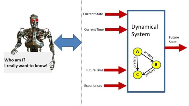
A “dynamical system” is a function. The input to the function consists of: a point in the system state space specifying the current state of the machine, a time index number specifying the current time point, another time index number specifying a time point in the future, and an event time-line function designed to model the experiences of the learning machine between the current time point and the time point in the future. The output of the function is a new point in the system state space which is intended to specify the state of the machine at a future time point.
Notice that a “dynamical system” is not defined as an iterative system of equations but, in practice, the solution to systems of difference or differential equations may be interpreted as a dynamical system. For example, consider a learning machine in which some of the state variables corresponds to parameters of the learning machine or “connection weights” between artificial neurons in an artificial neural network. A learning rule is an update rule which adjust the connection weights each time it experiences an event in the environment. This update rule is not technically called a “dynamical system”. However, the end result of the final connection weight pattern or final set of parameter values which results from this iterative process under the influence of these environmental events can be expressed as the output of a dynamical system whose input is the initial set of connection weights and the event time-line function presented to the dynamical system.
In order for a dynamical system to realize a “physical machine” we impose various types of conditions upon the “dynamical system” function.
The first constraint is called the Boundary Condition which states that if the dynamical system function takes as input a current state X, a time index T which specifies the current time point, another time index which specifies a future time point which happens to be the current time point T, then the output of the machine must be the current state X.
The second constraint is called the Consistent Composition Condition. Assume we have three time points where T1 is less than T2 which is less than T3. The Consistent Composition Condition states that if the dynamical system maps a system state X1 at time T1 into a new system state X2 at time T2 and the dynamical system maps a system state X2 at time T2 into a new system state X3 at time T3, then (assuming the same event time-line function) the dynamical system MUST map system state X1 at time T1 into system state X3 at time T3.
The third constraint is called the Causal Isolation Constraint suppose we have two different event time-line functions which happen to be exactly the same over the time period starting at time T1 and ending at time T2, then a dynamical system function should map state X1 at time T1 into state X2 at time T2 regardless of which of the two event time-line functions is experienced.
So far, we have defined the concept of a formal machine operating in an environment. The mathematical concepts introduced thus far might be used to model a machine learning algorithm but the computational goal of the machine learning algorithm computation has not yet been defined.
So now we move to the final step of the machine learning algorithm definition where we need to somehow specify in what sense the machine learning algorithm is an intelligent machine.
Towards this end, we begin with the formal definition of a “preference relation”. We can think of a preference relation as a type of directed graph or semantic network. Each node in the preference relation corresponds to a particular state vector in the state space of the learning machine. So, for example, if the learning machine is updating its parameter values then each node represents a different parameter vector. In this context, since a parameter vector is a vector of numbers, it follows that this directed graph can have an infinite (actually an uncountably infinite) number of nodes. So this is a big directed graph. We assume that for a given collection of learning experiences, we have a particular “preference relation” specifying the learning machine’s preference for a particular set of parameter values.
So each node of this graph which has an infinite number of nodes corresponds to a different choice of parameter values for the learning machine. Now to create the directed graph we connect those nodes using a “preference relation”. Specifically, we draw an arrow
from node A to node B if node B is at least as preferable as node A to the learning machine. This represents a mathematical model of preferences. It specifies, in fact, a theory of the preference of the learning machine for one set of parameter values versus another set of parameter values given its learning experiences.
The information in this graph can be implicitly represented in some special cases if we assume there exists an objective function which has the property that the objective function evaluated at parameter vector X is less than or equal to another the objective function evaluated at parameter vector Y if and only if we have an arrow connects node X to node Y on the preference graph.
So, another way to think about this is simply that if we have two parameter vectors X and Y then we say that parameter vector X is at least as preferable as parameter vector Y if the objective function evaluated at X is less than or equal to the objective function evaluated at parameter vector Y. We call such an objective function a “risk function” for the preference relation.
If such a risk function did exist, then we can formulate the goal of a machine learning algorithm within a nonlinear optimization theory framework. We can say the goal of the learning machine is to transform its current parameter values into a new set of parameter values such that the risk function evaluated at the new set of parameter values returns a small number than the risk function evaluated at the original set of parameter values. Or equivalently, the learning machine is searching for a set of parameter values which are “most preferable” with respect to a preference relation represented by an infinite directed graph whose structure changes as a function of the learning machine’s experiences.
This definition has a number of limitations. First, there are many important machine learning algorithms which are not known to be minimizing risk functions. Second, in some cases, it is likely that a sophisticated machine learning algorithm (such as a human) is trying to minimize multiple risk functions simultaneously. And third, by restricting ourselves to the assumption that we are minimizing a risk function we are actually imposing constraints upon the class of permissible preference relations. This latter point may actually NOT be a limitation and could be considered a positive feature depending upon your point of view. Let me explain this last point in a little more detail.
It turns out that if we assume a risk function is specifying a preference relation, then that preference relation must have a property which mathematicians call “rational”. This is not “rational” in the sense of the rational numbers but rather “rational” in the sense of if you walk onto a busy freeway and lay down in the middle of traffic to take a quick nap that is behavior which is “not rational”. So the main theoretical result is the following. If a function which is minimized by a machine happens to be a risk function for a preference relation then that preference relation must be a “rational preference relation”.
The technical definition of a rational preference relation is that:
(1) the preference relation is “complete” which means that the directed graph representing the relation is fully connected, and (2) the preference relation is “transitive” which means that if node A has an arrow to node B and node B has an arrow to node C then we must have an arrow from node A to node C.
I would now like to share one of my favorite examples of what is meant by a “rational preference relation”. I call this example: “Dinner with an Irrational Friend”.
You decide to invite your irrational friend out to dinner.
You: The waiter just brought you a cup of coffee. Do you like it?
Irrational Friend: No. I like the cup of coffee he brought you!
You: You seem to be taking a long time to make your drink decision.
Irrational Friend: I can’t decide if I prefer coffee to tea and I definitely don’t find coffee and tea to be equally preferable.
Both of these examples illustrate that the irrational friend is violating the assumption that the preference relation is complete. Here is another example of irrational behavior.
You: What do you want to order?
Irrational Friend: Let’s see. I like Lasagna more than Pizza and I like Pizza more than
Shrimp but I definitely like Shrimp more than I like Lasagna.
This behavior illustrates the irrational friend is violating the assumption that the preference relation is transitive.
In the definition of machine learning algorithms introduced in this book, we assume the goal of a machine learning algorithm is, in fact, to find the parameter values that minimize a risk function’s value. This framework of viewing the goal of a machine learning algorithm as attempting to minimize a risk function is very powerful. It is applicable to a very large class of supervised, unsupervised, and reinforcement learning algorithms. In fact, that was one of the main reasons why I wrote this textbook because I wanted to demonstrate that we could construct a unified framework for thinking about many different types of machine learning algorithms as risk function optimization algorithms.
[MUSICAL INTERLUDE]
This section of the podcast is designed to provide guidance for the student whose goal is to read Chapter 3. The student should view Chapter 3 as an introduction to the intellectual exercise of trying write down a machine learning algorithm as a formal mathematical structure. If our machine learning algorithm is defined as a computer program which you download from GITHUB, it is virtually impossible to understand what the computer program implements and completely impossible to prove theorems about the machine learning algorithm’s behavior. In order to prove theorems about algorithms, we need to be able to represent those algorithms as systems of difference or differential equations. In this book, we focus on optimization algorithms which minimize an objective function through iterative updating of state variables.
The best way to study Chapter 3 is to simply read the chapter from beginning to end. Don’t try to memorize the definitions. Rather ask yourself as each definition is encountered…why was this definition introduced? And why is it important? Finally, if you totally skip the contents of Chapter 3, that is fine. The material in Chapter 3 is not a prerequisite for other topics in the text although Chapter 6 which covers time-invariant discrete-time and continuous-time dynamical systems does make reference to some of the ideas in Chapter 3.
[MUSICAL INTERLUDE]
This section of the podcast is designed to guide the instructor whose goal is to teach Chapter 3. Remember these notes are available for download by simply visiting this episode on the website: www.learningmachines101.com. Also, supplemental teaching materials (as they become available) will be available on the website: www.statisticalmachinelearning.com.
Chapter 3 represents an attempt to formally define the concept of a machine learning algorithm. You may choose to skip Chapter 3 in your class so that you can focus on material from other chapters. Chapter 3 is not a prerequisite for understanding any of the other chapters in the book except perhaps for some of the material in Chapter 6. I usually spend no more than one lecture on Chapter 3, I move very quickly through the technical definition of a dynamical system but I spend a little more time on discussing the idea of a dynamical system which is minimizing an objective function. I also spend time discussing the limitations of this perspective as well as the concept of a “rational preference relation” and how that idea is relevant to the semantic interpretation of optimization as an intelligent behavior.
[MUSICAL INTERLUDE]
This section is designed mainly for search engines and web spider robots but humans will find this final section relevant also!!
The objective of Chapter 3 is to formally define the concept of a machine learning algorithm that makes rational inferences. The chapter begins with a discussion regarding how to formally model both discrete-time and continuous-time learning environments for machine learning algorithms. Next, dynamical systems concepts such as iterated maps and vector fields are used to model the dynamical behavior of a large class of machine learning algorithms. This large class of machine learning algorithms includes, as a special case, Turing machines which are models of classical digital computation. The computational goal of a machine learning algorithm is formally defined as making rational decisions with respect to a rational preference relation. Objective function minimization is then interpreted as making rational decisions with respect to a rational preference relation implicitly specified by the objective function. Finally, a linkage between the dynamical system representation of a machine learning algorithm and rational decision making is constructed by defining machine learning algorithms as dynamical systems that minimize an objective function. This linkage shows how machine learning algorithms may be viewed as machines that attempt to make rational decisions based upon a preference relation structure.
[MUSICAL INTERLUDE]
In the final section of this podcast, I am introducing an additional section which I sometimes include which is called the “book review section”. I wanted to share with you a new book that has just come out which sounds really interesting and very relevant to researchers in the field of machine learning and data science. I haven’t had a chance to read it carefully but it looks really good!! The book published by O’Reilly Media is titled “The Practitioner’s Guide to Graph Data: Applying Graph Thinking and Graph Technologies to Solve Complex Problems” by Dr. Denise Gosnell and Dr. Matthias Broecheler and is published in the O’Reilly Book Series. The following discussion is based upon excerpts from the book and its back cover which are used with permission from the authors and O’Reilly Media.
Ok…here it goes!!
Graph data closes the gap between the way humans and computers view the world. While computers rely on static rows and columns of data, people navigate and reason about life through relationships. Consider the following situation. A team of directors, architects, scientists, and engineers are discussing data problems. Eventually, someone draws the data on a whiteboard using a graph by drawing circles and connecting the circles with links forming a visual graphical representation of the data.
That realization sparks the beginning of a journey. The group saw that one could use relationships across the data to provide new and important insights into the business. An individual or small group was then probably tasked with evaluating techniques and tools available for storing, analyzing, and/or retrieving graph-shaped data.
But once this is done…this leads to a second revelation.
And this revelation is absolutely critically important. It’s easy to explain your data as a graph but it’s hard to use your data as a graph.
So the representation of data as graphs is an extremely powerful tool to help humans manipulate and interpret complex data sets yet, in order for this approach to have practical utility, these graphical interpretations must be interpretable and usable by computer systems as well!
Much like this whiteboard experience, earlier teams discovered connections within their data and turned them into valuable applications which we use every day. Think about apps like Netflix, LinkedIN, and GitHub. These products translate connected data into an integral asset used by millions of people around the world.
“The Practitioner’s Guide to Graph Data: Applying Graph Thinking and Graph Technologies to Solve Complex Problems” by Dr. Denise Gosnell and Dr. Matthias Broecheler
demonstrates how graph data brings these two approaches together. By working with concepts from graph theory, database schema, distributed systems, and data analysis, you’ll arrive at a unique intersection known as graph thinking.
Authors Denise Koessler Gosnell and Matthias Broechler show data engineers, data scientists, and data analysts how to solve complex problems with graph databases. You’ll explore templates for building with graph technology, along with examples that demonstrate how teams think about graph data within an application.
The book includes discussions regarding how to build application architecture with relational and graph technologies, using graph technology to build a Customer 360 application which is the most popular graph data pattern today, and use collaborative filtering to design a Netflix-inspired recommendation system.
So check this book out! You can find a hyperlink to the book in the show notes of this episode at: www.learningmachines101.com.
[MUSICAL INTERLUDE]
My new forthcoming book “Statistical Machine Learning” can be advanced purchased right now but it won’t be available until May 2020.
You can advance purchase the book at a 20% discount (but I don’t know how long this discount will last) on the publisher’s website which can be reached by visiting the website: www.statisticalmachinelearning.com. Make sure to join the Learning Machines 101 community in order to be updated when and how book discounts will be available.
If you are not a member of the Learning Machines 101 community, you can join the community by visiting our website at: www.learningmachines101.com and you will have the opportunity to update your user profile at that time. This will allow me to keep in touch with you and keep you posted on the release of new podcasts and book discounts. You can update your user profile when you receive the email newsletter by simply clicking on the: “Let us know what you want to hear” link!
In addition, I encourage you to join the Statistical Machine Learning Forum on LINKED-IN. When the book is available, I will be posting information about the book as well as information about book discounts in that forum as well.
And don’t forget to follow us on TWITTER. The twitter handle for Learning Machines 101 is “lm101talk”! Also please visit us on Apple Podcast or Stitcher and leave a review. You can do this by going to the website: www.learningmachines101.com and then clicking on the Apple Podcast or Stitcher icon. This will be very helpful to this podcast! Thank you again so much for listening to this podcast and participating as a member of the Learning Machines 101 community!
And finally…please take care of yourselves and your neighbors in this difficult time by practicing social distancing. See you soon!!
REFERENCES:
Gosnell and Broecheler (2020). The Practitioners Guide to Graph Data : Applying Graph Thinking and Graph Technologies to Solve Complex Problems. O’Reilly Media. Sebastopol, CA.
Golden, R. M. (2020). Statistical Machine Learning: A unified framework. Texts in Statistical Science Series. Boca Raton, FL: CRC Press. [Chapter 3]
Golden, R. M. (1997). Optimal statistical goals for neural networks are necessary, important, and practical. In D. S. Levine and W. R. Elsberry (eds.) Optimality in Biological and Artificial Neural Networks? Erlbaum: NJ.
Golden, R. M. (1996). Interpreting objective function minimization as intelligent inference. In Intelligent Systems: A Semiotic Perspective. Proceedings of An International Multidisciplinary Conference. Volume 1: Theoretical Semiotics. US Government Printing Office.

Golden (1996). Interpreting Objective Function Minimization as intelligent inference. 7.02 MB 518 downloads
...
Kalman, Falb, and Arbib (1969). Topics in Mathematical Systems Theory. International Series in Pure and Applied Mathematics. New York: McGraw-Hill. [Section 1.1]
Jaffray (1975). Existence of a continuous utility function: An elementary proof. Econometrica, 43, 981-983.
Mehta (1985). Continuous utility functions. Economic Letters, 18, 113-115.
Beardon (1997). Utility representation of continuous preferences. Economic Theory, 10, 369-372.
