Podcast: Play in new window | Download | Embed
Episode Summary:
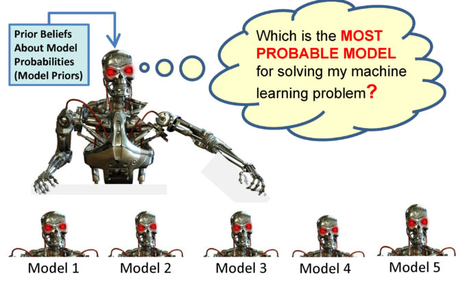
In this episode, we explain the proper semantic interpretation of the Bayesian Information Criterion (BIC) and emphasize how this semantic interpretation is fundamentally different from AIC (Akaike Information Criterion) model selection methods. Briefly, BIC is used to estimate the probability of the training data given the probability model, while AIC is used to estimate out-of-sample prediction error. The probability of the training data given the model is called the “marginal likelihood”. Using the marginal likelihood, one can calculate the probability of a model given the training data and then use this analysis to support selecting the most probable model, selecting a model that minimizes expected risk, and support Bayesian model averaging. The assumptions which are required for BIC to be a valid approximation for the probability of the training data given the probability model are also discussed.
Show Notes:
Hello everyone! Welcome to the 77th podcast in the podcast series Learning Machines 101. In this series of podcasts my goal is to discuss important concepts of artificial intelligence and machine learning in hopefully an entertaining and educational manner.
In the model selection problem you have two or more different models. For example, suppose you are trying to predict whether or not it will rain tomorrow based upon the temperature, humidity, and rainfall for the past seven days. This could be one model. Another model might try to predict whether or not it will rain tomorrow based upon only the temperature and rainfall measurements for the past month. You would like to figure out which of these two models will be more useful for predicting whether or not it will rain tomorrow.
In the previous episode 76th episode of Learning Machines 101, we discussed the Akaike Information Criterion for determining which of two competing probability models is the best model. In this 77th episode of Learning Machines 101 we will discuss the Bayesian Information Criterion for determining which of two competing probability models is the best model. Okay..spoiler alert!! I’m going to tell you one of the key points of this episode really quickly so this may ruin the suspense of the episode for you! One of the key points of this episode is that although the Akaike Information Criterion and Bayesian Information Criterion are algorithms which look very similar, the semantic criteria for selecting the model in these two cases is fundamentally different. The Akaike Information Criterion (also know as AIC) selects the model should be used when you want to select the model which has the smallest prediction error on TEST DATA. In contrast, the Bayesian Information Criterion provides a method for you to revise your prior beliefs regarding which model is most appropriate based upon the observed data and thus allows you to estimate the “probability your model is appropriate given the TRAINING data”. It’s really important to keep the semantic differences between these two model selection criteria clear because they are both easy to implement and they both penalize a model based upon the number of parameters in a model. If you don’t understand the mathematical theory behind these two model selection criteria you might think they are trying to do essentially the same thing but they each have complementary but fundamentally different model selection objectives.
To solve the model selection problem using the Bayesian Information Criterion we do the following. First, estimate the performance of your learning machine using one of the models using some training data. This is accomplished by finding the parameter values of your learning machine that make the observed data most probable. Such parameters are called maximum likelihood estimates and are described in Episode 55 of learning machines 101. Maximum likelihood estimation methods are very common in statistics and machine learning. Second, the prediction error of the learning machine is computed by figuring out the learning machine’s predicted probability of each training stimulus it observed. If the training stimuli are statistically independent, then the probability of the training data set is simply the product of the probabilities of the individual training stimuli in the training data set. The prediction error is defined as negative one multiplied by the natural logarithm of the probability of the training data set divided by the number of training stimuli.
Thus, as the learning machine adjusts its parameters to make the probability of the observed training data more likely, this prediction error tends to decrease. We will call this the negative normalized log-likelihood prediction error. This is actually a very commonly used prediction error in machine learning. Third, we are now going to compute a special term which is called the BIC or Bayesian Information Criterion penalty term. The BIC penalty term is defined as the number of free parameters in the model multiplied by the natural logarithm of the number of training stimuli and then divide this product by twice the number of training stimuli. The fourth step is to add the negative normalized log-likelihood prediction error term to the BIC penalty term to obtain what I call the “normalized BIC measure”. The BIC is defined as the normalized BIC measure multiplied by twice the number of training stimuli. The fifth step is to compute the BIC for each model and then select the model which has the smallest BIC.
Note that since all of the models are fit to the same data set, you will get the same model selection results regardless of whether you use BIC or the normalized BIC measure. I like the normalized BIC measure because it is not sample-size dependent.
So the Bayesian Information Criterion is relatively easy to compute. Let K be the number of free parameters in the model. Let N be the number of data records. Let E be the negative normalized log-likelihood prediction error. Then the BIC is simply given by the formula 2N E + K log (N). Compute this formula for each of your models and choose the model with the smallest BIC.
Simple right! The problem is that because this is so simple to implement and use there is a lot of potential for not using the Bayesian Information Criterion correctly resulting in wrong solutions to the model selection problem. In fact, I would not be surprised if the majority of scientists and engineers are incorrectly using the Bayesian Information Criterion because they do not have a clear understanding of what the BIC is designed to estimate and the specific conditions under which the BIC estimates are valid.
In this podcast, we will explain the concepts of the Bayesian Information Criterion carefully to better understand its strengths and limitations. We will explicitly provide assumptions for the BIC to hold. In the show notes of the podcast, I will provide references to the literature which describe explicit assumptions required for the BIC to be valid and key theorems which reveal the specific semantic interpretation of the BIC.
So the first step of this process is to understand in a precise way what is the semantic interpretation of the BIC. Some researchers state that the semantic interpretation is to find a parsimonious model that fits the data. The BIC penalty term generates a smaller penalty when the model has fewer free parameters. In particular, the BIC penalty term which you add to the average prediction error is given by the formula: number of free parameters multiplied by the logarithm of the sample size divided by twice the sample size. As the sample size becomes large, the effects of the BIC penalty term become negligible. However, if the model has lots of free parameters then the BIC penalty term tends to increase the model selection criterion value making that model is less attractive.
But what is the logic behind the magic of this ritual? Why don’t we multiply the model’s prediction error by 7 which is a much more magical number and then add the number of free parameters? Why don’t we square the number of free parameters of the model and then add that to the square root of the model’s prediction error? All of these formulas are equally consistent with the intuitive qualitative concept that we are trying to find a model which fits the data which has as few parameters as possible. Also how do we count free parameters? Suppose I have a Gaussian probability model with two parameters: a mean and a variance. I then decide I want to rewrite the mean as the product of 8 parameters which yields a Gaussian probability model with 9 parameters. Does that change the BIC? Why is this not valid? In order to understand the answers to these questions which will be revealed shortly, it is necessary to re-examine the fundamental semantic interpretation of the BIC. At the beginning of the podcast, I basically gave you the essential idea but now in this section we want to develop this semantic interpretation a little more systematically.
Let’s begin by discussing the concept of a PROBABILITY MODEL. Most learning machines can be interpreted as seeking parameter values so that they can estimate the probability of events in their environment. The probability of an environmental event is calculated by the learning machine using the learning machine’s probabilistic model of its environment. Technically, a probability model is a set of probability distributions which are typically indexed by a choice of parameter values. But less formally, we can think of the learning machine as adjusting its parameter values based upon its experiences in the world so that the learning machine’s expectations about the probability of specific events in its environment “best approximates” the actual probability of those events in its environment. In many real-world situations,There does not exist a probability distribution in the learning machine’s probability model which EXACTLY specifies the probability distribution which actually generated the training data. In such cases, we say the learning machine’s probability model is “misspecified” with respect to it’s statistical environment in order ot calculate the probability of a probability model we first compute the probability of the training data given the probability model. To do this, we need two ingredients.
For our first ingredient, we need a well defined probability model whose elements are indexed by some parameter vector. We compute the probability of the first training stimulus and compute the probability of the second training stimulus. Since the training stimuli are assumed independent we can multiply these two probabilities to get the probability of observing both of the training stimuli. If we observe N training stimuli, then we compute the probability of observing each training stimulus for a given set of parameter values and then multiply all N of those probabilities together to obtain the probability of observing the N training stimuli given the parameter values of the model. When the parameter values are chosen to maximize the likelihood of the training data, then the parameter values are called “maximum likelihood estimates”. These concepts are introduced and discussed in Episode 55 of the learning machines podcast series.
For our second ingredient, we need a “parameter prior” for that probability model which specifies the probability of good quality parameter values. The parameter prior concept is discussed in Episode 55 of Learning Machines 101. The essential idea is that parameter prior specifies the probability that a particular parameter value or a particular set of parameter values is appropriate. The parameter prior is obtained based upon prior knowledge of what the parameter values should look like BEFORE we have observed any training data. So, for example, suppose you were modeling the height of an individual as a Gaussian random variable with some mean and some variance. The parameter prior for the mean would probably range from 0 feet to 8 feet while the parameter prior for the variance would probably be about 36 feet. Since we don’t really know much about the parameter values for the learning machine before the learning process, such parameter priors are typically called “vague priors” since they instantiate weak probabilistic knowledge constraints.
The probability of the training data given the probability model is called the “marginal likelihood”. It is computed by multiplying the probability of the training data given one particular choice of model parameter values multiplied by the prior parameter probability of that choice of parameter values plus the probability of the training data given another particular choice of parameter values multiplied by the prior parameter probability of that second choice of parameter values and so on. So essentially we are INTEGRATING the joint probability of the training data and the parameter values given the probability model over all possible parameter values in the probability model. The resulting multidimensional integral is called the “marginal likelihood” and it represents the probability of the DATA given the MODEL.
It’s typically very difficult to compute this. One can use the Monte Carlo simulation methods but another way is to use a BIC approximation which provides a formula for estimating the marginal likelihood. In particular, if we exponentiate the -N multiplied by the negative normalized log-likelihood evaluated at the maximum likelihood estimates plus the BIC penalty term, then this provides an approximation for the marginal likelihood for large sample sizes.
Once the Marginal Likelihood is obtained, then the “most probable” model can be found using Bayes rule. This requires specifying another prior which is called the “model prior” which represents the probability that a particular probability model is appropriate before any data has been observed by the learning machine. Let the “evidence” for a particular defined as the marginal likelihood for that model multiplied by the probability of that model as specified by the model prior. Then the probability of a model is simply the evidence for that model divided by the sum of the evidence of all of the models under consideration. If you are just interested in identifying the “most probable” model then you can just use the “evidence measure” and select the model which has the greatest evidence.
The basic idea here is that you get a prediction from each model in your set of models and then you generate a prediction not from a particular model but from the entire set of models by multiplying the prediction of the first model by the probability of the first model given the training data and then adding that to the product of the prediction of the second model multiplied by the probability of the second model given the training data and then adding that to the product of the prediction of the third model multiplied by the probability of the third model given the training data and so on. In many cases, Bayesian model averaging will give much higher quality predictions. There are theoretical reasons for this (I will give some references at the end of the podcast) and there is lots of empirical work which shows this is a good idea as well.
In order to correctly apply the Bayesian Information Criterion, certain assumptions must hold. Fortunately, these assumptions hold in most situations but unfortunately these assumptions are not carefully checked before applying the BIC in practice by most engineers and scientists.
Let’s briefly go over a set of sufficient conditions for BIC to be applicable. First, we will assume that the N training stimuli are the outcomes of sampling N times with replacement from a large but finite set of feature vectors. Second, the measure of prediction error computed for each feature vector is assumed to be a smooth function of the parameter values so that the second derivatives of the prediction error per training stimuli with respect to the parameter values are continuous. Also the prediction error should be a continuous or piecewise continuous function of each feature vector. Third, parameter estimates are computed by minimizing the negative log-likelihood function for a data set so that the parameter estimates are maximum likelihood estimates. Maximum Likelihood estimation is discussed in Episode LM101-055 of Learning Machines 101. Fourth, it will be assumed that the parameter estimates will converge to a unique set of parameter values as the number of training stimuli gets larger and larger. Fifth, the derivative of the prediction error per training stimulus evaluated at the maximum likelihood estimates is called the gradient stimulus prediction error vector which has q elements. Compute the outer-product of each gradient stimulus prediction error vector and then average all N outer-products. The resulting matrix is called the B matrix. The eigenvalues of B should be empirically checked to make sure that they are converging to finite positive numbers. Sixth, the second derivative of the prediction error per training stimulus which is a q-dimensional matrix is computed and evaluated at the maximum likelihood estimates. These N second derivatives are averaged to obtain a matrix called the A matrix. We also need to empirically check that the eigenvalues of A are converging to finite positive numbers.
The above assumptions are applicable to a large class of important probability models including linear regression models and logistic regression models. They are also applicable to highly nonlinear regression models and deep learning models which satisfy these assumptions.
In practical applications of the Bayesian Information Criterion, some of these assumptions are probably violated. Thus, even though the computer program used calculates the Bayesian Information Criterion the resulting estimates of the probability of the model given the observed data are not valid. These are crucial assumptions which are often satisfied in practice when the parameter estimates are converging to a locally unique stable solution. However, even though these assumptions might often be satisfied in practice, it is important to understand when these assumptions fail and thus invalidate the methodology.
One major problem in common usage of the Bayesian Information Criterion is that I have rarely seen engineers or scientists report the eigenvalues of the A and B matrices are converging to positive numbers suggesting that these important conditions are not properly checked. These assumptions are closely related to the issue of having “stable” parameter estimates with respect to the parameters in your model. For example, suppose you had a linear regression model with 1000 free parameters and you had two data points. You will find in this case that the assumptions that the eigenvalues of A and B are all positive will be violated. As another example, suppose we consider the previously stated example where we have a Gaussian probability distribution with some mean and some variance and we rewrite the mean of the Gaussian distribution as the product of eight free parameters. The resulting Gaussian probability model has 9 free parameters but this particular way in which we have defined the parameters of the Gaussian probability model will violate the assumption that the eigenvalues of the A matrix are positive. Therefore, this is an illegal parameterization.
Another challenge in applying the Bayesian Information Criterion occurs with highly nonlinear smooth regression models. For example, consider a deep learning network such as discussed in Episode LM101-023 where the negative normalized log-likelihood prediction error is constructed so that it is a smooth function of the parameter values. Highly nonlinear regression models and deep learning networks often have multiple saddlepoints, flats, and strict local minimizers. In order for the BIC to work, the maximum likelihood estimates must converge to a particular local minimizer of the expected negative normalized log-likelihood prediction error as the number of training stimuli becomes large. The BIC analysis fails if we converge to a saddlepoint or a flat plateau on the prediction error surface. If we are converging to a particular strict local minimizer even if it is not a unique global minimizer, then the analysis is valid. The semantic interpretation in this case is simply that the BIC is estimating the probability of a “local probability model” whose parameter space is defined as a small ball containing the strict local minimizer.
Another way to think of this local probability model condition that we are at a strict local minimizer is that if we perturb the parameter estimates slightly in any way then when the sample size is really large the average prediction error needs to increase. Also it is worth commenting that when we have a very complicated model with multiple strict local minimizers we are really using the BIC to compare “local probability models” defined on different regions of the original parameter space!
There have been a number of recent important advances in Bayesian Information Criterion theory. Although the BIC is actually valid for comparing possibly misspecified models, one can develop a higher-order version of BIC which provides better quality results for smaller samples. These more advanced versions of BIC are discussed by Lv and Liu in a 2014 article published in the Journal of the Royal Statistical Society. In addition, I have recently developed with my colleagues a version of BIC which estimates the most probable model given a typical data set rather than the most probable model given the observed data set. This variation of BIC which I call XBIC is helpful for avoiding the estimated probability of a model from becoming dependent upon the training data (see paper by Golden et al. 2015 listed at end of this podcast shownotes). In addition, references to the recent work of Lv and Liu and more classical references associated with the analysis of BIC are provided. Check out all of these references by going to the website: www.learningmachines101.com and checking out the references at the end of the show notes of this Episode.
Thank you again for listening to this episode of Learning Machines 101! I would like to remind you also that if you are a member of the Learning Machines 101 community, please update your user profile and let me know what topics you would like me to cover in this podcast. You can update your user profile when you receive the email newsletter by simply clicking on the: “Let us know what you want to hear” link! As a member of the Learning Machines 101 community you will also receive an email approximately once a month designed to let you know when this month’s podcast has been released.
If you are not a member of the Learning Machines 101 community, you can join the community by visiting our website at: www.learningmachines101.com and you will have the opportunity to update your user profile at that time. You can also post requests for specific topics or comments about the show in the Statistical Machine Learning Forum on Linked In.
From time to time, I will review the profiles of members of the Learning Machines 101 community and comments posted in the Statistical Machine Learning Forum on Linked In and do my best to talk about topics of interest to the members of this group!
And don’t forget to follow us on TWITTER. The twitter handle for Learning Machines 101 is “lm101talk”!
Also please visit us on ITUNES and leave a review. You can do this by going to the website: www.learningmachines101.com and then clicking on the ITUNES icon. This will be very helpful to this podcast! Thank you so much. Your feedback and encouragement are greatly valued!
Keywords: Bayesian Information Criterion, BIC, Schwarz Information Criterion, Model Selection Criterion, Marginal Likelihood
Related Podcasts:
- LM101-055: How to Learn Statistical Regularities using MAP and Maximum Likelihood Estimation
- LM101-076: How to Choose the Best Model using AIC or GAIC
Further Reading:
- Burnham, K. P. and Anderson, D. R. (2010). Model Selection and Multimodel Inference: A Practical Information-Theoretic Approach. Springer-Verlag. https://www.amazon.com/Model-Selection-Multimodel-Inference-Information-Theoretic/dp/0387953647/
[Most podcaster listeners will probably like the Burnham and Anderson book since the here the primary focus is on applying these ideas in practice. Includes a good discussion of Bayesian Model Averaging.] - Claeskens, G.; Hjort, N. L. (2008), Model Selection and Model Averaging, Cambridge University Press. Cambridge Series in Statistical and Probabilistic Mathematics. [See Chapter 3. This chapter has a nice mix of practical real-world examples and references to the rigorous mathematical statistics literature. Some parts should be accessible to general public while other parts require more advanced statistical modeling background.]
- Evans, M. and Swartz, T. (2005). Approximating Integrals via Monte Carlo and Deterministic Methods. Oxford Statistical Science Series. [ See Section 4.4 for a high quality discussion of the asymptotic approximations associated with BIC].
- Konishi and Kitagawa (2008). Information Criteria and Statistical Modeling. See Chapter 9.
Clear theoretical introduction to BIC.
https://www-springer-com.libproxy.utdallas.edu/us/book/9780387718866. - Schwarz, G. (1978). Estimating the dimension of a model. The Annals of Statistics, 6, 461-464. [Classic reference for BIC/SIC].
- Lv and Liu (2014). Model selection principles in misspecified models. Journal of the Royal Statistical Society, Series B, 76, pp. 141-167. [Recent important developments of BIC].
- Golden, Nandy, Patel, and Viraktamath (2015). A Laplace approximation for approximate Bayesian Model Selection. Presented at the 2015 Advances in Approximate Bayesian Inference NIPS 2015 Workshop (http://www.approximateinference.org/2015/accepted/)
- Hoeting, Madigan, Raftery, and Volinsky (1999). Bayesian Model Averaging: A Tutorial. Statistical Science, 4, 382-417. [Good comprehensive tutorial on Bayesian Model Averaging for statisticians]
