Cartoon describing statistical learning with priors.

Podcast: Play in new window | Download | Embed

LM101-055: How to Learn Statistical Regularities using MAP and ML Estimation

Episode Summary:

In this rerun of Episode 10, we discuss fundamental principles of learning in statistical environments including the design of learning machines that can use prior knowledge to facilitate and guide the learning of statistical regularities.

Show Notes:

Hello everyone! Welcome to the tenth podcast in the podcast series Learning Machines 101. In this series of podcasts my goal is to discuss important concepts of artificial intelligence and machine learning in hopefully an entertaining and educational manner.

The nature versus nurture problem corresponds to the problem which tries to disentangle what parts of our knowledge are due to our experiences (that is “nurture”) and what parts of our knowledge of the world are due to our genetic disposition (that is “nature”).

Cognitive-neuroscientists now understand that the majority of animal and human knowledge is acquired neither purely by biological growth specified by genetic disposition or purely by learning but rather is a process involving complex interactions between both of these processes. Babies are born with biological brain structures which have some parameters which are highly modifiable by experience while other properties of these biological brain structures are not modifiable by experience at all. Some structural features of the brain change in a dramatic way as a function of both experience and the age of the organism, while others are programmed to evolve relatively independently of the environment. Babies are not 11^th century tabula rasa machines with blank minds waiting for experiences to be imprinted but they are also not genetically pre-programmed with all of the knowledge they will require to survive in their environments. Both nature and nurture interact in a complex manner throughout the growth and development of humans and animals to create biological intelligence.

In this podcast episode, we discuss fundamental principles of learning in statistical environments. Specifically, what is a statistical environment? How can we design a learning machine that can learn within such an environment? How can we build into the statistical learning machine “genetic dispositions” to facilitate and guide learning processes. In short, we are investigating the “nature versus nurture” problem for statistical learning machines.

Consider the problem of designing a learning machine which has a particular probabilistic model of reality. Specifically the learning machine believes that certain events occur with certain frequencies in the world. A probabilistic law for the learning machine would be a collection of beliefs which indicate the expected percentage of times that different events in the world would occur. Before learning begins, the learning machine has a large collection of probabilistic laws as well as expectations regarding which laws are most likely to be applicable. This large collection of probabilistic laws will be called the learning machine’s probabilistic model of its environment. The machine’s expectations regarding which laws are most likely to be applicable are called the priors. The goal of the learning process is to select a probabilistic law from the learning machine’s probabilistic model which “best matches” the environmental probabilistic law. The events that are generated from the environmental probability law correspond to a particular sequence of outcomes of the DGP or Data Generating Process.

To illustrate these ideas, let’s discuss these concepts using the idea of a probabilistic logical rule which was introduced in Episode 7 and Episode 8.

In Episodes 7 and 8, we talked about the idea of a probabilistic logical rule of the form:

IF event X occurs, THEN event Y occurs with probability P

The probability P is called a “probability parameter” and the probability parameter for each rule is adjusted during the learning process so that the learning machine makes more intelligent inductive inferences.

The set of all possible probabilistic logical rules where each probabilistic logical rule has its own specific number assigned to its probability parameter is an example of a “probability model”. The “priors” in this case could be another collection of probabilities indicating which probabilistic logical rules are most likely. The priors are “hints” provided to the learning machine about its environment before any learning has taken place. And finally, the learning process involves selecting the appropriate set of probabilistic logical rules for a given collection of observed data.

Alternatively, we can also think of the machine’s probabilistic model of its environment as its “genetic disposition” or the “nature process” which is also specified by the “priors”. While the matching process where the correct probabilistic law for representing the machine’s statistical environment is learned by adjusting the “probability parameters” is called the “nurture process”.

Suppose we go to Las Vegas and decide to play a game of roulette where you spin a roulette wheel and a little ball will drop into one of the slots. You place a bet that the little ball will fall into a particular slot. For example, you might bet the little ball falls into a red slot with a certain probability. This seems like a statistical environment but it could also be viewed as a deterministic environment. We could alternatively view the behavior of the roulette wheel as a complicated deterministic nonlinear dynamical system. We would use the laws of physics to describe the behavior of the wheel, air friction, the initial force exerted by the guy that spins the wheel, the air pressure at the casino, and so on. Thus, this is another example where the exact same physical process can be viewed as either generating random outcomes or deterministic outcomes.

What do we mean by a deterministic view of reality? This was the dominant view of 16^th century or even 13^th century physics which talked about a “clockwork of reality”. The basic idea of the “clockwork” or “deterministic” view of reality is that once we have discovered all of the physical laws of the universe we can make predictions of all possible events into the distant future. According to this view, if we understand the laws of physics then we can make predictions about how frequently we will see a solar eclipse or how frequently a comet will pass near the earth. With respect to human behavior, we might be able to make predictions about someone’s behavior if we could identify the set of logical rules that govern their behavior.

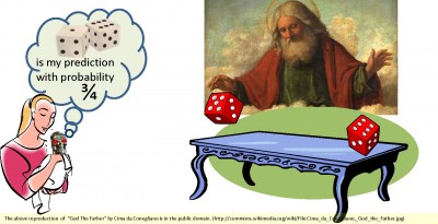
An alternative viewpoint is the probabilistic view of reality. In the 21^st century, the theory of Quantum Mechanics was introduced which took probabilistic statements regarding the behavior of atomic particles as fundamental. For example, quantum mechanics makes probabilistic statements about the position and velocity of an electron but does not make deterministic predictions. Einstein did not like the probabilistic view of reality and greatly favored the deterministic viewpoint with his famous statement “God does not play with dice.”

When we throw a die, we observe one out of 6 possible outcomes. This seems like a random event since you have an equal chance of observing either: 1, 2, 3, 4, 5, or 6 dots. On the other hand, we can view this as a deterministic event which is not random at all. In this latter case, we would have to build a complex nonlinear model of the instantaneous force applied to the die, the orientation of the die when the force was applied, the air viscosity, the force of gravity, and other factors. This would be an extremely complicated mathematical model but it would be deterministic. This suggests that even if God did play with dice that doesn’t mean that the world is necessarily a world of random events.

Thus, one could argue that the issue of whether God plays with dice is not a discussion about reality but rather a discussion about the appropriate choice of how to model reality. There is nothing which is fundamentally deterministic or probabilistic about a game of checkers or a coin of toss. The outcome of a coin toss could be viewed as a random event. Or, the outcome of a coin toss could be viewed as a deterministic event without any randomness at all. This leads us to a crucial point. A particular environment is not intrinsically random or deterministic. We can, however, model exactly the same environment as either behaving according to deterministic or probabilistic laws.

It is important to emphasize that the probabilistic perspective is not restricted to modeling gambling games but is applicable to many other types of environments associated with machine learning problems. Many types of machine learning problems can be described in terms of trying to discover the probabilistic law which determines the observed expected frequency of the roll of a weighted die.

We assume that God or equivalently the Environment plays with dice in the following manner in order to generate the weather. The Environment has these three dice and each die is weighted in a different manner so that one side is more likely to come up than another side. If it is a “cloudy day”, then the Environment picks the die called the “cloudy today die” and rolls that die. If the outcome of the roll of the cloudy today die is “rainy”, then the Environment makes tomorrow a rainy day. If the outcome of the roll of the cloudy today die is “sunny” then the Environment makes tomorrow a sunny day. Thus, in this example, we really do have God playing with dice! Unfortunately, we do not have access to the three dice that the Environment is using to generate weather patterns. If we knew how those dice were weighted, then we would always be able to calculate the exact expected frequency tomorrow’s weather would be: rainy, sunny, or cloudy given our knowledge of today’s weather.

We will assume that although we do not have the 3 dice that the Environment uses to generate the weather, we have prior knowledge that the Environment is using the “rainy today”,“a sunny today”, and “cloudy today” dice. We are interested in estimating the expected frequency that a particular outcome of a die roll is observed. The goal of the learning machine is to figure out the weightings of each of these three dice. These “weightings” can be viewed as probabilistic logical rules as discussed in Episode 7 and Episode 8 of this podcast series.

Specifically, we seek probabilistic logical rules of the form:

IF today is a sunny day, THEN the probability that tomorrow will be a rainy day is 3/10

IF today is a rainy day, THEN the probability that tomorrow will be a rainy day is 9/10.

In order to predict the weather, a learning machine would simply record each day whether yesterday’s weather was: rainy, sunny, or cloudy. In addition, the learning machine would record whether today’s weather was: rainy, sunny, or cloudy. Using this information, the learning machine could deduce statistics such as: the percentage of times a sunny day follows a rainy day or the percentage of times a cloudy day follows a rainy day. These statistics could then be used to estimate the expected frequency of these various types of events. With this information, probabilistic logical rules can be derived for predicting the likelihood of different environmental events.

This is the essential idea behind a statistical learning machine. Essentially all statistical learning machines work in this way. When you are using your smart phone and your smart phone makes suggestions regarding who you want to phone, your smart phone is typically using some sort of statistical learning algorithm similar to the approach we have described. When your photo editor make suggestions regarding how the pictures in your picture library should be sorted and categorized, your photo editor is using a statistical learning algorithm of this type as well. Voice recognition systems learn statistical regularities peculiar to your personal specific dialect and modify themselves accordingly.

Note, however, this solution to the learning problem assumes that the learning machine has available large amounts of data from which the percentage that particular events occur in the environment can be reliably calculated.

In real life we usually don’t have the luxury of observing large amounts of data and then making a decision. Often we are forced to make decisions as data arrives so how can we learn in situations where we are in the process of collecting data?

Consider the case where a learning machine is trying to predict the weather and the learning machine has not yet seen any data. If we want the learning machine to make a prediction, the learning machine needs to have a collection of probabilistic laws. The goal of learning is to select the appropriate probabilistic law which can then be used to calculate the observed expected frequency of environmental events.

Before the learning machine has been exposed to any training experiences, it also may be required to make inferences. In order to deal with such situations, the learning machine is also provided a “prior” which is the “prior probability” that a particular probabilistic law is applicable. We can think of “priors” as analogous to specifying the likelihood of a particular genetic disposition.

So, for example, the learning machine might assume that before it has the opportunity to be presented with any training data that all of the probabilistic laws that are potentially learnable by the machine are equally likely. This assumption is called the assumption of the uniform prior. This would be a good assumption for some places in the world. However, for other places in the world such as San Diego, the learning machine might be biased with some other prior that attaches a greater likelihood to probabilistic laws that predict sunny day events more frequently.

Humans and animals have numerous genetic dispositions. That is, tendencies to learn some behaviors more easily than others.

Consider the problem of teaching a dog to sit. Suppose you tell your dog to sit, and then you give your dog a treat. The dog quickly learns that when it sits, that it gets a treat. Now suppose you tell your dog to chase a rabbit, the dog chases the rabbit, and then you give your dog a treat. So this type of learning is totally consistent with the ideas that we have discussed. Inside the dog’s mind is a die which is labeled “chase rabbit” and when the dog chases a rabbit the likelihood that when that die is rolled the dog will observe the outcome of “get treat” is very high.

Ok…now we illustrate the concept of “genetic disposition”. It is much more difficult to train your dog using treats to NOT chase a rabbit. Dogs are wired up to chase rabbits. It is very difficult to untrain dogs to chase rabbits although it can be done. This is an example of the dog’s genetic disposition which corresponds to a probabilistic prior overriding or impeding the dog’s learning experiences.

Using the concept of a prior, the learning machine can make predictions about the likelihood of different events before it has learned anything!!

Now let’s consider the initial stages of the learning process where the learning machine has observed a small amount of data. Perhaps the learning machine has been watching the weather for three days. The first day was sunny, the second day was cloudy, and the third day was cloudy. The learning machine should reason that this corresponds to the situation where the Environment:

(1) rolled the die named “sunny today” and observed the outcome “cloudy” and THEN

(2) rolled the die named “cloudy today” and observed the outcome “cloudy”

Using this information, the learning machine would note that since a cloudy day follows a sunny day once, it would make sense to assign the weighting of the “sunny today” die such that it comes up “cloudy” 100% of the time. In addition, the weighting of the “cloudy today” die should be adjusted so that when clouday day die is rolled the outcome “cloudy” is observed 100% of the time.

Or, in other words, we have learned the rules:

IF today is a sunny day, THEN tomorrow will be a cloudy day with 100% certainty.

IF today is a cloudy day, THEN tomorrow will be a cloudy day with 100% certainty.

Now assume a sunny day follows a cloudy day three times and a rainy day follows a cloudy day once, then the chances of a rainy day following a cloudy day are estimated to be three times as likely as the chances of a sunny day following a cloudy day. That is, a rainy day follows a cloudy day 75% of the time.

Using this observed data, the learning machine would derive the following probabilistic logical rules:

IF today is a cloudy day, THEN tomorrow will be a rainy day with probability 75%.

IF today is a cloudy day, THEN tomorrow will be a sunny day with probability 25%.

Here, we see the learning machine is using the percentage of times that an event occurs in its environment as a prediction of the likelihood that the event will occur in the future. This type of reasoning is called “Maximum Likelihood Estimation”.

It is important to note that maximum likelihood estimation is not formally defined as using observed frequencies of events to estimate the chances of occurrences of events. Instead, maximum likelihood estimation is formally defined as finding the probabilistic law that makes the observed data most likely. In the special case where the learning machine can exactly represent its environment, then it can be shown that maximum likelihood estimation is equivalent to estimating the probability something occurs by the frequency that it occurs.

More generally, however, in the real world the learning machine does not have the luxury of observing large amounts of data. And, in addition, in the real world the learning machine’s probabilistic model of reality will always have some fatal flaws. The more general definition of maximum likelihood estimation allows us to deal directly with both of these problems.

The more general definition of maximum likelihood estimation states that given a collection of data, the learning machine should use its assumptions about its probabilistic world to calculate the probability of the observed data. Next, the learning machine “learns” about its environment by trying to adjust its probabilistic model of the world so that it assigns larger probabilities to events in the world which have been observed. Thus, the learning machine is able to apply the maximum likelihood estimation methods in situations where only small amounts of data are present and in cases where the machine’s probabilistic model of its world is not perfectly accurate.

The problem of investigating inference and learning when your probabilistic model of the world does not contain the true probabilistic law is called the “model misspecification problem”.

Maximum likelihood estimation learning theory does not require the assumption that the learning machine’s probabilistic model is correct. Suppose we defined the goal of learning is to exactly learn the expected frequencies of events in the environment. If the learning machine’s model of the environment is flawed then it may not be capable of exactly representing the true expected frequencies of events in its environment. Thus, with this definition of learning, it is not possible to interpret learning within environments when the learning machine’s probabilistic model of reality can not perfectly represent its probabilistic environment.

In the real world, all models are flawed. Thus, we would not prefer a theory of learning which requires that the learning machine’s probabilistic model can always perfectly represent its environment. Fortunately, the maximum likelihood estimation learning framework avoids this problem. And, in the special case where the learning machine’s probabilistic model can represent its statistical environment perfectly, maximum likelihood estimation is equivalent to estimating probabilities by their observed frequencies.

So, to summarize, maximum likelihood estimation totally ignores the use of “priors” and calculates the probabilistic law that makes the observed data most likely.

And, maximum likelihood estimation defines a “good inductive inference” as an inference made using a probabilistic law that makes the observed data most likely regardless of the amount of data and regardless of the accuracy of the machine’s probabilistic model of reality.

Such a definition is reasonable but can be improved even further!

Specifically, computing the probabilistic law that makes the observed data most likely seems less appropriate than computing the “most probable probabilistic law” given the observed data. This alternative idea is called “Maximum A Posteriori Estimation” (MAP Estimation).

Suppose that we want to find the probabilistic law that is most likely given the observed data? That is, solve the MAP estimation problem. The solution to the MAP estimation problem is quite fascinating.

When you work out the mathematics of MAP estimation, it turns out that in the initial stages of MAP estimation learning the learning machine is biased to follow its “priors” while in the later stages of MAP estimation learning, the learning machine is based to ignore its “priors” and becomes a maximum likelihood estimation learning machine!

We thus can think of MAP estimation as the mathematician’s solution to the “nature” versus “nurture” problem. MAP estimation is a mathematical procedure which precisely shows how the “nature” and “nurture” factors trade off against one another in a MAP estimation statistical learning machine!!

So, to summarize, we’ve talked about a variety of issues. All of these issues are fundamentally important to many machine learning algorithms.

First, we noted that environments that might seem intrinsically deterministic can be viewed as probabilistic and environments that might seem intrinsically probabilistic can be viewed as deterministic. This point was made to emphasize that probabilistic view of reality is just as real as a deterministic view of reality. Second, we introduced the idea of MAP estimation which can be defined as selecting the “most probable” probabilistic law based upon the experiences of the learning machine to date.

Before any data is observed, the “most probable” probabilistic law is specified by the “priors”. A “prior” is the learning machine’s expectation that a probabilistic law is appropriate and this expectation is given to the learning machine before the machine is provided with learning experiences.

Then, in the early stages of learning, MAP estimation combines the “priors” and the system’s experiences in the world to compute the “most probable” probabilistic representation of reality.

After large amounts of data have been observed, the MAP estimation theory of learning tends to ignore and discount the effects of prior knowledge and focuses upon only the system’s experiences in the world in order to compute the “most probable” probabilistic representation of reality. And, in the rare but important special case, where the learning machine is capable of adequately representing its probabilistic environment, it can be shown that the “most probable” probabilistic representation of reality is, in fact, that representation of reality where the learning machine’s calculation that of the probability of an event is exactly equal to the expected frequency of that event in the learning machine’s environment.

LM101-055: How to Learn Statistical Regularities using MAP and Maximum Likelihood Estimation (Rerun)

LM101-055: How to Learn Statistical Regularities using MAP and ML Estimation

Episode Summary:

Show Notes:

Further Reading:

Leave a Reply Cancel reply