What robot is thinking when it classifies a dog image as the word dog.

Podcast: Play in new window | Download | Embed

LM101-030: How to Improve Deep Learning Performance with Artificial Brain Damage (Dropout and Model Averaging)

Episode Summary:

Deep learning machine technology has rapidly developed over the past five years due in part to a variety of factors such as: better technology, convolutional net algorithms, rectified linear units, and a relatively new learning strategy called “dropout” in which hidden unit feature detectors are temporarily deleted during the learning process. This article introduces and discusses the concept of “dropout” to support deep learning performance and makes connections of the “dropout” concept to concepts of regularization and model averaging.

Show Notes:

Hello everyone! Welcome to the thirtieth podcast in the podcast series Learning Machines 101. In this series of podcasts my goal is to discuss important concepts of artificial intelligence and machine learning in hopefully an entertaining and educational manner.

Recently, I attended the International Conference on Learning Representations 2015 which was followed by the Artificial Intelligence in Statistics 2015 Conference in San Diego. The ICLR conference might be described as a conference which has a strong focus on the problem of “deep learning” using primarily an empirical methodology. On the other hand, the Artificial Intelligence in Statistics conference or AISTATS emphasizes theoretical methodologies. In future podcasts, I will discuss and review aspects of these conferences which have influenced my thinking in profound ways. I will also provide background information relevant to understanding this review. You can access the papers which were presented at the ICLR conference or the AISTATS conference by visiting the website: www.learningmachines101.com

While attending both of these conferences, I’m always on the lookout for some common technique that everybody is doing and obtaining great results in learning machine design. One such technique is called “dropout” which is a relatively new idea which recently surfaced in the machine learning community. At the conference, I noticed that many of the talks and posters which were using deep learning techniques on large-scale networks were employing “dropout regularization”. Let me quickly comment on a few examples of a few talks and presentations that I observed which used this technique.

At the ICLR conference, there was a featured talk by Karen Simonyan and Andrew Zisserman titled “Very Deep Convolutional Networks for Large-Scale Image Recognition”. In this talk they used a convolutional neural network architecture such as I described in podcast episode 29 which had approximately 16-19 layers of connection weights or equivalently layers of units. This type of network architecture has approximately 100 million free parameters. The network was trained with a database of 1.3 million images and tested using 100,000 novel images. In this data set, there are 1000 different classes of images and the convolutional network has to figure out how to assign a particular image to a particular class. Using a super-computer setup with four NVIDIA Titan Black GPUs, training a single convolutional network took approximately 2 or 3 weeks of continuous computing time. Using this methodology, the research team secured second place in the ImageNet 2014 Large Scale Visual Recognition Challenge (a competition designed to identify the top algorithms in machine learning) so basically the performance was state-of-the art. They used L2 regularization and dropout regularization which will be explained shortly. In my opinion, the crucial idea which makes a network such as this work correctly is the convolutional network representation with maxpooling and rectified linear units which is why I devoted Episode 29 to explaining these concepts. However, many other factors including “dropout” are important.

The presentation by Tom Le Paine, Pooya Khorrami, Wei Han, and Thomas Huang from the Beckman Institute for Advanced Science and Technology was titled “An Analysis of Unsupervised Pre-Training in Light of Recent Advances”. In Episode 23 of this podcast series, I described the concept of using “unsupervised pre-training” to support learning in deep learning neural networks. The basic idea was that you first train the first layer of the deep learning neural network with an unsupervised learning rule and then fix those parameters so they can not change. Then you add a second layer of units and train the second layer of units and do not train the first layer of units. Then you fix the parameters of the second layer of units so they can not change and you add a third layer of units. After the entire multi-layer network is trained in this way, all of the parameter values of the multi-layer network are allowed to change simultaneously during the learning process using a supervised learning algorithm. The parameter values generated during the unsupervised learning process provide excellent guesses to support learning for the supervised learning algorithm. These deep learning ideas are discussed in detail in Episode 23 of this podcast series.

Basically, because we are using a gradient descent type algorithm which is very sensitive to initial conditions for objective functions with multiple saddlepoints and local minima (see Episode 16 for more details), this greedy unsupervised pre-training procedure helps bootstrap the system by presenting the system with a succession of learning problems to facilitate learning. Human learning has similar characteristics to this type of strategy. Before one learns the nuances of a very complex skill such as playing world-class chess or playing world-class racquetball, one begins by learning very basic skills. These basic skills then provide a foundation for the development of more complex skills. Complex skills are often not directly learned by humans.

More recently, however, rectified linear units have played an important role in solving many deep learning problems and, in fact, researchers discovered that if they used rectified linear units it was not necessary to do pretraining. Thus, many of the researchers at this machine learning conference were using deep learning without pretraining as described in Episode 23. Because the concept of a rectified linear unit is so important for solving deep learning problems, I discussed the concept of “rectified linear units” previously in my last podcast Episode 29.

The paper by Tom Le Paine and his colleagues re-examines whether pretraining is really necessary given recent advanced in deep learning which include rectified linear units as well as other new ideas such as dropout.

In this paper, one of the natural image datasets CIFAR-10 consists of 60,000 32 x 32 pixel images with 10 class categories and 6,000 images per class. In this paper, 50,000 of the images were used for training and 10,000 of the images were used for testing. They used a convolutional neural network architecture with three layers of units followed by an additional layer of hidden units followed by the output unit layer. The convolutional filters in the first two layers were 5 x 5 while the filters in the third layer were 3 x 3. There were also 2 x 2 max pooling layers after the first two convolutional layers which essentially cut the feature map size in half. These concepts are explained in detail in my last podcast Episode 29. The classification performance of their system on the test data was approximately 86% which was not the best of all algorithms used to solve this image classification problem but was definitely in the top 80% percentile in a competition where its competitors were state-of-the-art machine learning algorithms. In other words, it did pretty well!

They then used variations of this architecture to explore the effects of pretraining and dropout. Basically, they found that although performance could be quite good without pretraining when rectified linear units are used, the pretraining method described in Episode 23 helps performance for supervised learning. They also showed that “dropout” also increased performance.

So now that we have established that “dropout” is important…what is dropout?

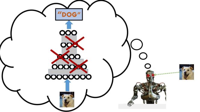
The basic idea of dropout regularization is most easily described in the context of an adaptive learning machine. Assume that the goal is to train an adaptive learning machine which has a layer of hidden units. That is, the input units which receive the input pattern feed their outputs to the hidden units who feed their responses, in turn, to the output units of the learning machine. In adaptive learning, a training stimulus is presented to the learning machine and its parameters are updated. The dropout regularization version of adaptive learning is based upon the following procedure. First, a training stimulus is presented to the learning machine. Second, we randomly select a subset of hidden to be temporarily deleted from the learning machine for the purpose of this learning trial. It is assumed that each hidden unit has the same probability of being deleted at that learning trial. So, for example, suppose the probability of deleting a hidden unit from the model is equal to ½ and there are three hidden units in the learning machine. The first training stimulus is presented to the learning machine on the first learning trial. We now want to decide which of the three hidden units should be deleted so we flip a fair coin three times for the current learning trial. If the first coin toss outcome is heads, then hidden unit 1 is deleted. If the second coin toss outcome is heads, then hidden unit 2 is deleted. If the third coin toss outcome is heads, then hidden unit 3 is deleted. the deletion of a hidden unit means that all of the inputs and all of the outputs of the deleted hidden unit must be deleted as well. So, if the outcome of the three coin tosses, was: tails, heads, heads then this would mean that only the first hidden units and its incoming and outgoing connections would be used to compute the gradient descent parameter update for the network. Then the second training stimulus is presented and perhaps when we flip the coin three times that all coins come up tails. This would imply that we would do a regular gradient descent step which would involve an additional update to the connections for the first hidden unit as well as updates to the remaining hidden units in the network.

Although the dropout algorithm seems straightforward, it also seems a little non-intuitive. Why would deleting hidden units randomly and then putting them back improve predictive performance on the test sample? Wouldn’t this just make the task harder? To understand this issue, let’s discuss the concept of “regularization” which we have talked about in various other episodes of Learning Machines 101.

Despite the fact that large data sets are often used to train these learning machines and the convolutional neural network methodology provides a highly structured network, the resulting learning machine might have thousands of free parameters. When a learning machine has many extra free parameters, there is always the danger of overfitting. This means that the learning machine might not only learn important statistical regularities in the environment which are common to all data sets but will also learn silly statistical regularities which are peculiar to the specific data set which is being used to the train the learning machine. One approach used to avoid overfitting problems is to impede the learning process making it more difficult for the silly statistical regularities to become “settled” in the learning machine. For example, weight decay is a widely used method in machine learning for addressing the overfitting problem. This approach modifies the learning rule so that the parameters of the learning machine tend to “decay” or “fade out” and converge to zero. A commonly used approach to implement weight decay is to add an additional term to the objective function minimized by the learning machine. This additional term is called a regularization term. If the regularization term is the sum of the squares of the current parameter values of the learning machine, then gradient descent on this type of regularization term will cause the parameters of the learning machine to fade out towards zero. This is called L2- or “ridge” regularization in statistics. If the regularization term is the SQUARE ROOT of the sum of the squares of the current parameter values of the learning machine, then gradient descent on this type of regularization term will also cause the parameter of the learning machine to fade out towards zero but the convergence to zero will be more rapid for the smaller parameter values. This latter type of regularization is called L1-regularization or “lasso” regularization in statistics. L1 lasso regularization appears to be more widely used than L2 ridge regularization in the statistical machine learning community. As a direct consequence of L1 or L2 regularization parameter values which do not contribute significantly to predictive performance are forced towards the value of zero thus reducing the complexity of the network. Or to summarize these ideas in a more concise way, regularization constraints of these types make it “harder” to learn statistical regularities which tends to “filter out” inconsistent weak statistical regularities and bias the system to learn the more consistent strong statistical regularities.

Many machine learning researchers consider “dropout” to play a role similar to L1-regularization and L2-regularization. By picking a hidden unit and its connections at a particular learning trial to be temporarily ignored with some probability P for that learning trial, it is claimed that this tends to force the hidden units to work more independently and not be as “dependent” upon other hidden units. The following analogy might help explain this phenomenon.

Imagine a big company which manufactures cars where the boss of the company is worried that many of the workers in the company are not pulling their own weight and are “slackers”. The basic idea of “L1”-regularization (i.e., ridge regression) and “L2”-regularization (i.e., lasso regression) is that one fires employees in such a manner so as to maintain approximately the same productivity levels. So, if the company has 100 employees and manufactures 100 widgets in one month, then L1 or L2 regularization tries to fire 20% of the employees while maintaining the same level of widget production. This means that the 20% least productive employees are eliminated. The employees in this example correspond to the parameter values of the learning machine and the number of cars manufactured per month is a measure of predictive performance for a learning machine.

Dropout regularization, on the other hand, focuses more upon optimizing the organizational structure of the company. Imagine that in order to produce a car there are various intermediate steps that need to be accomplished. For example, there might be several groups at the company who manufacture wheels while several groups at the company manufacture brakes and several other groups who manufacture engines. In dropout regularization, the company gives a vacation day to each group at the company with some probability every day of the year. This might seem great but it is expected that the level of productivity of the company be optimized despite the fact that everybody at this company enjoys a frequent vacation day. This means that individual groups need to not be “dependent” upon other groups at the company and need to make sure they are efficient at pulling their own weight. The groups of employees in this example who manufacture different car parts correspond to the hidden units in the learning machine and the company’s productivity corresponds to the learning machine’s predictive performance.

But there is, in fact, a deeper level of understanding of what is going on here. In fact, I think that the concept of “dropout” as a type of regularization is actually confusing the issue. It makes more sense to think of “dropout” as implementing a system of “model averaging” which I will now explain briefly.

Most researchers tend to focus on finding the “best” learning machine which seems, at first glance, to be a smart and reasonable type of goal. We call this the “model selection” problem in machine learning. But is this goal of the model selection problem really that great? To illustrate the potential flaws with this perspective, suppose that you select 10 of your friends with the goal of figuring out who is the “best automobile driver” by having them all complete a specially designed automobile driving test. Then you will designate that friend to be your official driver on a cross-country road trip!! Note that each of the 10 friends corresponds to a different complex learning machine with millions of free parameters. The objective function which these learning machines are trying to minimize is computed by evaluating their driving test score. Ok…back to the driving test!!

To achieve this goal you design the automobile driving test and have your 10 friends drive the course. As a result of the automobile driving test, you find that 2 of your friends are horrible drivers, 5 of your friends are good drivers, and 3 of your friends were the best automobile drivers. In fact, the 3 best drivers had exactly the same score on the driving test. But even though they had exactly the same score on the driving test, this does not mean that the complex collection of skills necessary for driving for each of your 3 friends who were excellent automobile drivers are equivalent. Sally is really good at driving fast and passing people without causing accidents. Jim drives at a good, safe, consistent pace. Bill has very fast reaction times and can rapidly assess a situation and make a good driving move. Although the driving test has given each of these three drivers equivalent driving scores, the driving styles and capabilities of each of these three drivers are certainly not equivalent. One could say that since they are all equally good drivers, let’s just pick one at random to be the driver for the cross-country road trip but this might not be the best possible strategy.

Sally might be a better choice for driving long stretches of roads such as those in Kansas where you drive for miles really fast and you have to pass a truck or two along the way. Jim might be a better choice for driving along treacherous mountain roads. And Bill might be the best driver choice for driving in east-coast traffic jams. All three of these drivers had the same excellent score on the driving test but because they are very complex learning machines with complex skill sets, their performance in the same situation will not at all always be equivalent! Ideally (and this would make the road trip more fun anyway), you should invite: Sally, Bill, and Jim to join you on a cross-country road trip and let the three of them decide who is the best driver for a particular part of the journey!!

This example illustrates the basic idea of “model averaging”. Rather than trying to pick the model which has the smallest prediction error, the idea is to realize that if you are building complex learning machines with thousands or millions of free parameters which are learning very complex tasks that you may end up with hundreds or thousands of learning machines which tie for first place as far as prediction error yet it doesn’t make sense when you have identified 1000 learning machines which have the smallest prediction error to just choose one at random and use that learning machine. The smart strategy is to use all 1000 learning machines and combine their results.

Another example is suppose you wanted to solve a complicated engineering problem. So you identify the top 5 scientists and engineers who are experts in this area and can solve that complex engineering problem. All 5 of these scientists and engineers are eager to work on the problem. Assuming you had the relevant financial resources, it would be totally illogical for you to try to figure out which of the 5 was the best person for the job and just hire that one person! It would make more sense to hire all 5 individuals and have them work as a team to solve the complicated engineering problem. This is another example of the advantages of “model averaging” over “model selection”.

Now let’s return to the “dropout” strategy and re-interpret what is going on from a model averaging perspective. The recent paper by Srivistiva et al. (2014) published in the Journal of Machine Learning Research does just this although the model averaging interpretation was also emphasized by Hinton and his colleagues in 2012. Hyperlinks to both of these papers can be obtained by visiting the transcript of this episode at: www.learningmachines101.com.

The key idea involves visualizing the dropout for a learning machine with only three hidden units by assuming that the learning process is essentially training eight different learning machines with the original set of training stimuli. This is because each of the three hidden units can be temporarily deleted or kept so if compute 2³ that is equal to 8! Thus, each of the eight learning machines corresponds to a particular selection pattern indicating which hidden units and their connections should be ignored at a particular learning trial and which hidden units and their connections should not be ignored.

The first learning machine only uses the first hidden unit, the second learning machine only uses the first two hidden units, the third learning machine might use the first and third hidden units, and so on. We then use the original set of training stimuli to train all eight learning machines but we constrain the connections among the learning machines so that if the connections from the input units to the first hidden unit are updated for one learning machine then they are updated for all other learning machines which include the first hidden unit in their network architecture.

In other words, rather than thinking of one network architecture where the probability of a hidden unit is ignored at a learning trial is some constant probability, instead, we visualize the learning problem as training a large army of learning machines where the size of the army is an exponential function of the number of hidden units. So for example, with three hidden units there are 2³ or 8 learning machines but with 30 hidden units there are 2³⁰ or over 1 billion learning machines! At each learning trial, instead of picking which hidden units in a layer of 30 hidden units to temporarily delete, we pick one of the 1 billion learning machines at random which corresponds to a particular choice of which of the 30 hidden units should be temporarily deleted. Then we use the training stimulus to update the weights of that learning machine. Then after we have done this, we make similar weight changes all members of the billion-strong army of learning machines which have the same active hidden units.

The testing phase is a little tricky because it is clearly computationally challenging to present a test stimulus to 1 billion training machines and then compute the average response across all 1 billion training machines. Dropout has a heuristic way of adjusting the weights during the test phase which is designed to provide a computationally easy way to approximate this average response. The details of this procedure can be found in the dropout review articles in the transcripts of this episode. Although I have never used the standard procedures, I don’t recommend them based upon theoretical considerations.

Instead I recommend an enhanced Monte Carlo Averaging version of “dropout” as described in Srivistiva et al. (2014) in Section 7.5 which compares a Monte Carlo Averaging version of dropout with the standard dropout method. The Monte Carlo Averaging algorithm is still computationally very simple and I believe you would get much better results. The concept is as follows. First, even though we would like to apply the test input to all 1 billion learning machines and then average the outputs we agree that is too computationally expensive in many cases. Second, what we are going to do is to select a certain number of learning machines at random. For example, we might select 50 out of the 1 billion learning machines at random where the probability of selecting a learning machine is equal to the probability of selecting a particular pattern of hidden units to temporarily ignore. We then simply average the outputs of these 50 learning machines with the idea that the average will closely approximate the average for 1 billion learning machines. We can even estimate the standard error of this approximation if we choose to do so. In practice, the algorithm is even simpler than what I have just described. All we do is pick a pattern of hidden units to temporarily ignore (just as we do during the regular dropout learning process) and record the output of the learning machine. Then we pick another pattern of hidden units and generate an output. Then we pick another random pattern of hidden units to keep and generate an output. Then we average these outputs!

To summarize, dropout is commonly referred to as a regularization strategy but in fact it is probably best viewed as a crude approximation to a model averaging strategy. Model averaging is an important and complex topic and actually deserves its own podcast episode. but I will provide a very brief introduction here. Eventually we will have a special podcast on model averaging, Bayesian model averaging, and Frequentist model averaging.

Thank you again for listening to this episode of Learning Machines 101! I would like to remind you also that if you are a member of the Learning Machines 101 community, please update your user profile.

You can update your user profile when you receive the email newsletter by simply clicking on the: “Let us know what you want to hear” link!

Or if you are not a member of the Learning Machines 101 community, when you join the community by visiting our website at: www.learningmachines101.com you will have the opportunity to update your user profile at that time.

From time to time, I will review the profiles of members of the Learning Machines 101 community and do my best to talk about topics of interest to the members of this group!

Also consider joining the “Statistical Machine Learning Forum” group on LinkedIn! Your are encouraged to post comments about episodes at: www.learningmachines101.com or comments at the “Statistical Machine Learning Forum” group on LinkedIn. In addition to responding to your comments, those comments might be used as the basis for a future episode of “Learning Machines 101”!!

And finally, I noticed I have been getting some nice reviews on ITUNES. Thank you so much. Your feedback and encouragement is greatly valued!

Keywords: Dropout, Regularization, Model Averaging, Model Selection, Ridge Regression, Lasso Regression, Deep Learning, Convolutional Neural Networks, Feature Discovery, Hidden Units, Rectified Linear Units, Image Classification

LM101-030: How to Improve Deep Learning Performance with Artificial Brain Damage (Dropout and Model Averaging)

LM101-030: How to Improve Deep Learning Performance with Artificial Brain Damage (Dropout and Model Averaging)

Episode Summary:

Show Notes:

Further Reading:

Leave a Reply Cancel reply