Example of a deep learning neural network implementing a value function for playing checkers.

Podcast: Play in new window | Download | Embed

LM101-062: How to Transform a Supervised Learning Machine into a Value Function Reinforcement Learning Machine

Episode Summary:

This 62^nd episode of Learning Machines 101 discusses how to design reinforcement learning machines using your knowledge of how to build supervised learning machines! Specifically, we focus on Value Function Reinforcement Learning Machines which estimate the unobservable total penalty associated with an episode when only the beginning of the episode is observable. This estimated Value Function can then be used by the learning machine to select a particular action in a given situation to minimize the total future penalties that will be received. Applications include: building your own robot, building your own automatic aircraft lander, building your own automated stock market trading system, and building your own self-driving car!!

Show Notes:

Hello everyone! Welcome to the sixtieth-second podcast in the podcast series Learning Machines 101. In this series of podcasts my goal is to discuss important concepts of artificial intelligence and machine learning in hopefully an entertaining and educational manner.

In supervised learning, the learning machine is provided with explicit information regarding the correct response for a given input pattern. In unsupervised learning, the learning machine is simply provided input patterns without any explicit feedback from the environment. Reinforcement learning is an interesting combination of unsupervised and supervised learning methods which corresponds to the case where the learning machine interacts with its environment and the environment provides occasional minimal feedback regarding how the learning machine is performing without providing the learning machine with information regarding the correct response for a given environmental event. Reinforcement learning algorithms have been discussed in this podcast series in Episodes 2, 48, 49, 59, 61 which can be found on the official website for Learning Machines 101: www.learningmachines101.com .

A recent example of Deep Reinforcement Learning is described in Episode 59 of Learning Machines 101 which learns from experience without a teacher how to successfully play ATARI video games. In such games, the player often can apply a control mechanism to shoot various types of characters and when a character is shot then the incremental reward for shooting that particular agent is provided to the player. The total score for the player is the sum of these incremental rewards. A reference to the Deep Q Learning with Experience Replay Neural Network is provided in the show notes of this episode. In addition, I have provided a video link so you can watch the neural network learn to play the ATARI video game from experience!!!

In this episode, we will provide explicit details regarding how you can design your own reinforcement learning machine based upon your favorite supervised learning algorithm! Examples of supervised learning algorithms include favorite linear regression, logistic regression, nonlinear regression, or feedforward deep learning neural network. I will show you how you can modify your existing favorite supervised learning algorithm so that it can solve reinforcement learning problems!

The episode is organized as follows. First, we will briefly review solving a supervised learning problem by minimizing average prediction error. This problem was discussed previously in Episodes 14, 15, 23, 29, 41, 51, of learning machines 101 but we will review this again briefly. Solving the supervised learning problem by minimizing average prediction error model includes as important special cases: (1) linear regression models, (2) logistic regression models, (3) multinomial logistic regression models, (4) nonlinear regression models, and (5) multi-layer feedforward deep learning neural networks with many layers of processing.

After we have discussed the supervised learning problem we will discuss how to modify that solution to solve the reinforcement learning problem. We illustrate these ideas with respect to the problem of learning to play checkers but these ideas can be generalized to a variety of problems including robot control, making trades on the stock market, and training self-driving cars.

In a supervised learning problem, one provide the learning machine with both an input pattern and the desired response to the input pattern. The goal of the learning process is to generate the desired response for a given input pattern. In addition, suppose we present the system with an input pattern that it has never seen before, then we would like it to generate a reasonable response to that input pattern based upon its past experiences.

Suppose we want to build a machine learning algorithm to play checkers. A checkerboard consists of 64 squares. Only 32 squares are actually used in the game since neither you or your opponent are allowed to place checker pieces on half of the squares. On some of the squares are regular checker pieces which belong to either yourself or your opponent. In addition, some squares contain special checker pieces called “kings” which have additional freedom of movement. The first step in building a learning machine to play checkers is to represent the checkerboard as a list of numbers which is called a “vector”. This might be accomplished as follows. First, take a look at the first square on the checkerboard in which a player is allowed to place a checker piece, if no checker piece is present then the first 4 elements of the vector are set equal to zero. If the first square on the checkerboard has the learning machine’s checker piece and it is not a king then make the 1^st element of the vector equal to 1 and the 2^nd , 3^rd, and 4^th elements of the vector equal to zero. If the first square on the checkerboard has the learning machine’s checker piece and it is a king, then make the 2^ndelement of the vector equal to 1 and the 1^st, 3^rd , and 4^th elements of the vector equal to zero. The 3^rd and 4^th elements of the vector are defined in a similar way to specify the presence of the opponent’s checker piece and whether or not it is a king. This defines the first 4 elements of the vector representing the first square of the 64 square checkerboard. This coding process is then repeated for the remaining 31 squares where playing pieces can be placed. This yields a vector with 32 multiplied by 4 elements or equivalently 128 numbers in the binary vector consisting of ones and zeros. We will call such a vector a “checkerboard state vector”.

Now suppose we want to teach our learning machine to play checkers using “supervised learning”. This means that we present the learning machine with an input checkerboard state vector and we also tell the learning machine which of the permissible legal moves for that given input checkerboard state vector is the correct choice. The learning machine then uses this information to adjust its parameter values such that given a particular input checkerboard state vector it can estimate the probability that a particular permissible legal move should be chosen to win the game. The prediction error for making a particular permissible legal move is then defined as negative one multiplied by the logarithm of the machine learning algorithm’s estimate that the probability that move was the correct choice. Thus, if the machine learning algorithm predicts the desired move is correct with probability one then the prediction error is the negative logarithm of 1 which is equal to zero. On the other hand, if the machine learning algorithm predicts the desired move is correct with a very small probability p then the prediction error is given by the negative logarithm of p which is a very large positive number. A “softmax” or “multinomial logit regression model” might be considered for this implementation which is constrained in such a manner that the current input checkerboard state vector assigns a probability of zero to illegal moves.

So, more generally, we can think of a supervised learning machine as generating a predicted response from a given function of an input pattern and parameter values. This function can be chosen to implement a linear regression model, a logistic regression model, or a multi-layer feedforward nonlinear neural network. This is essentially a nonlinear regression modeling problem. In the checkerboard example, the input pattern would be a checkerboard position and the desired response would be a good legal move on the checkerboard which would enhance your winning position. The learning machine has parameter values which can be adjusted. Different choices of parameters values correspond to different strategies for making moves.

The goal of supervised learning is to find the parameter values which minimize some measure of average prediction error. Average prediction error can be computed in a variety of different ways. For example, the prediction error could be defined as the negative logarithm of the predicted probability that a choice is correct as in our checker playing example or the prediction error could be defined as the square error difference between the desired response and the predicted response for a given input pattern and the learning machine’s parameter values. I provide the exact equations illustrating these ideas in a handout which can be downloaded from the reference section of this podcast.

Of course the obvious difficulty with the above approach is that the correct choice for a given input checkerboard state vector is often not available. Not only is it unknown by the novice who is learning to play checkers, it is also unknown by the expert!

The goal of a reinforcement learning machine is to predict an appropriate output pattern vector given an input pattern vector and a ”hint” about the nature of the output pattern vector. Typically, the terminology ”reinforcement learning” assumes a temporal component is present in the machine learning problem. Thus, the entire feature vector consists of some features which represent the state of the learning machine at different points in time while other elements of the feature vector provide non-specific feedback in the form of a hint regarding whether the learning machine’s behavior over time was successful. For example, suppose a robot is learning a complex sequence of actions in order to achieve some goal such as picking up a coke can. There are many different action sequences which are equally effective and the correct evaluation of the robot’s performance is whether or not the robot has successfully picked up the coke can. Furthermore, this reinforcement is non-specific in the sense that it does not provide explicit instructions to the robot’s actuators regarding what they should do and how they should activate in sequence. And, the problem is even more challenging because the feedback provided to the robot after an action sequence is executed. This situation is similar to the problem of making trades in the stock market where you are making a sequence of trades and the consequences of those trades are not appreciated until the end of an episode. The situation is also similar to the problem of learning to play checkers where you make a sequence of moves in the checker game but the consequences of that move sequence are not observed until the end of an episode. Note that an episode for a checker game could correspond to an entire game of checkers where the final outcome of the episode of the checker game is who won the game but it could also correspond to a sequence of ten moves within the checker game where one’s success in the game is evaluated over ten move increments. The concept of mini-episodes is also relevant in other areas of reinforcement learning such as robot control, aircraft landing, and stock market trading. So, in the following discussion, the terminology episode might correspond to a long complex sequence of events such as investing a large sum of money in the stock market or a sequence of mini-episodes corresponding to how the investment should be treated over a shorter time span. Or, in the robot control example, an episode could correspond to the action sequence of picking up a coke can but it also might correspond to a component mini-episode where the robot grasps a coke can or another mini-episode where the robot lifts a coke can.

Ok…so our first assumption which we need to extend the concept of supervised learning to reinforcement learning is that episodes are independent and identically distributed. This is an overly strong assumption but it has the benefit of allowing us to get robust results in a relatively easy and straightforward manner. These episodes can be mini-episodes and they can vary in length. It is assumed that an episode always starts with some initial environmental state which is observed by the learning machine and this initial state is independent and identically distributed. The subsequent states in the episode occur with probabilities dependent upon the initial state. In our example, the initial environmental state corresponds to the checkerboard state vector which is the state of the checkerboard. Then we assume the learning machine takes some action based upon a “policy” which is also known as a “control law”. The “policy” is a function which the learning machine uses to calculate an action based upon a given environmental state. In this example, the action would be legal checkerboard move taken with respect to the current environmental state which is the current state of the checkerboard. The environment then generates a new environmental state based upon the learning machine’s action. In this example, that new environmental state would be the state of the checkerboard generated by the opponent of the learning machine as a consequence of the move chosen by the learning machine’s opponent. In addition, we assume the presence of a reinforcement penalty function which generates an incremental reinforcement penalty associated with the transition from one environmental state to another. The reinforcement penalty function is assumed to lie at the interface between the learning machine’s actions and the environment.

So, to summarize, reinforcement learning is viewed as taking place with respect to a sequence of independent and identically distributed episodes. Each episode begins with an environmental state which occurs with some probability. Then the learning machine generates an action with some probability which depends upon the current environmental state. Then then environment generates a new environmental state with some probability which depends upon the previous environmental state and the learning machine’s previous action. This process continues until the end of the episode. The total reinforcement received for an episode is a weighted sum of the incremental reinforcement penalties received throughout the episode. The goal of the reinforcement learning process is to minimize the expected reinforcement penalty per episode based upon the probability of occurrence of a particular episode.

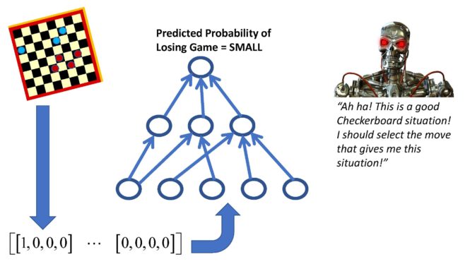
Ok now we will discuss how to transform any nonlinear regression model (including linear regression and multi-layer deep neural network models) into a Value Function Reinforcement Learning Machine. So first it is important that we are clear what we mean by a Value Function. A Value Function takes as input the initial state of an episode and returns a number which specifies the expected total penalty reinforcement received over the course of the entire episode based upon observing only the first initial state of that episode! In the context of the checkerboard game, the input pattern for the supervised learning machine would be a checkerboard pattern and the desired response would NOT be the correct move. Instead, the desired response would be a numerical representation of the probability that you will lose the game if you leave your opponent with that checkerboard position after you make your checkerboard move. This probability of losing the checkerboard game is an example of what we have been calling the expected total reinforcement penalty for an episode given only the initial state of the episode.

If we could estimate such a Value Function, then it could be used to help us solve reinforcement learning problems in the following way. We simply generate several possible actions for a given environmental state and then evaluate the Value Function at the different environmental states generated by the different possible actions. We then choose the action which leads to the Value Function which has the smallest value. So, for example, suppose we had a Value Function which provided us with the future expected reinforcement penalty for a given state of a checkerboard and it is our turn to make a move. Also assume we have only three possible moves but this approach can be generalized to handle more possible moves in a straightforward manner. We try the first possible move which changes the checkerboard state and we evaluate our Value Function and get the number 14, then we try the second possible move which changes the checkerboard state and get the number 6, then we try the third possible move which changes the checkerboard state and get the number 20. So we conclude that we should take move 2 since that move will minimize the total expected penalty reinforcement we will receive into the future.

Once the Value Function has been learned it can be used to predict the distant future consequences of making a particular move for a particular checkerboard position, taking a particular trade in stock market trading situation, or generating a particular amount of thrust in a situation where one is attempting to land a spacecraft. Thus, this type of learning machine does not actually learn to generate actions. It simply learns a Value Function which can then be used to guide the selection of actions in different situations.

So now we know how to use the Value Function if we had such a function. But how do we design the learning algorithm for our supervised learning machine? We assume that during the learning process the learning machine gets to observe the first two environmental states of each episode. Also recall that we are also assuming that the episodes are independent and identically distributed. And we additionally assume that the sum of all penalty reinforcement increments received in an episode is approximately equal to the total penalty reinforcement received in the episode.

So here is the key idea which is a little tricky. We evaluate the Value Function evaluated at the first environmental state of the episode which is the sum of all future reinforcement increments and subtract from that the Value Function evaluated at the second environmental state of the episode. This yields a prediction of the expected incremental reinforcement to be received when the second environmental state follows the first environmental state of the episode. Since the incremental reinforcement obtained from the transition from the first to second environmental state is observable we can use the discrepancy between the predicted incremental reinforcement derived from evaluating the Value Function and the observed incremental reinforcement to estimate a prediction error.

Then we can adjust the parameters of the Value Function to minimize this prediction error which characterizes the discrepancy between the predicted and observed incremental reinforcement penalty.

In practice, the PREDICTED incremental reinforcement penalty received for a particular transition from the FIRST environmental state of an episode to the SECOND environmental state of the episode is given explicitly by subtracting a percentage of the Value Function evaluated at the second environmental state from the Value Function evaluated at the first environmental state. This percentage is called the “discount factor”. Intuitively, this implies that the penalties associated with environmental states near the end of an infinitely long episode should be negligible. Another consequence of this assumption is that when the discount factor is close to 0%, then this corresponds to the case the observed incremental reinforcement penalty for transitioning from one environmental state to another is a good approximation for the entire reinforcement penalty to be received in the distant future. Alternatively, when the discount factor is close to 100% this corresponds to the case where Value function evaluated at the first environmental state representing the total cumulative future reinforcement minus the Value function evaluated at the second environmental state representing the total cumulative reinforcement accumulated from the second state of the episode yields a prediction of the incremental reinforcement to be received when the learning machine transitions from the first environmental state to the second environmental state.

For example, one could define the prediction error as the observed incremental reinforcement penalty received from observing the transition from the first to the second environmental state of an episode minus the predicted incremental reinforcement penalty. The predicted incremental reinforcement penalty would be the Value Function evaluated at the first environmental state of the episode and the learning machine’s current parameter values minus the discount factor multiplied by the Value Function evaluated at the second environmental state of the episode and the learning machine’s current parameter values. The sum of the squares of the prediction errors could then be used to estimate the mean square prediction error for the learning machine for a given choice of parameter values.

Then, gradient descent or accelerated gradient descent methods such as described in Episode 31 of Learning Machines 101 can then be used to derive a learning rule which minimizes this objective function. As described in Episode 31, such methods are based upon picking an initial guess for the parameters of the learning machine, adjusting the parameters based upon a given training stimulus, then observing the next training stimulus, and updating the parameters again. And there you have it!!! We have shown how to build a Value Function Reinforcement Learning Machine using a Supervised Learning Machine Algorithm.

I want to emphasize that this podcast was designed to provide more technical details than I typically include in my podcasts so I have provided explicit formulas for reference purposes in the show notes of this episode which include concise descriptions of the relevant mathematics so that you can immediately implement and explore these ideas!!!

Next time I hope to share with you another large class of important reinforcement learning algorithms called Policy Gradient Reinforcement Learning algorithms!!!!

Thank you again for listening to this episode of Learning Machines 101! I would like to remind you also that if you are a member of the Learning Machines 101 community, please update your user profile and let me know what topics you would like me to cover in this podcast.

You can update your user profile when you receive the email newsletter by simply clicking on the: “Let us know what you want to hear” link!

If you are not a member of the Learning Machines 101 community, you can join the community by visiting our website at: www.learningmachines101.com and you will have the opportunity to update your user profile at that time. You can also post requests for specific topics or comments about the show in the Statistical Machine Learning Forum on Linked In.

The technical mathematical notes for this episode will be posted on the Statistical Machine Learning Forum in LinkedIn. In addition, the technical mathematical notes can be downloaded from the show notes of this episode if you are a member of the Learning Machines 101 community! Feel free to post questions and comments in the Statistical Machine Learning Forum regarding this special post or other posts!!

From time to time, I will review the profiles of members of the Learning Machines 101 community and comments posted in the Statistical Machine Learning Forum on Linked In and do my best to talk about topics of interest to the members of this group!

And don’t forget to follow us on TWITTER. The twitter handle for Learning Machines 101 is “lm101talk”!

And finally, I noticed I have been getting some nice reviews on ITUNES. Thank you so much. Your feedback and encouragement is greatly valued!

Protected: LM101-062 Technical Memo: Implementing Value Function Reinforcement Using A Nonlinear Regression Model

This technical memo describes how to implement a value function reinforcement learning algorithm using a nonlinear regression model of your choice.

Enter Password to Download:14 Downloads

Keywords: Reinforcement Learning, Supervised Learning, Stock Market, Robot Control, Game playing, Value Function, Q Learning, Deep Reinforcement Learning

LM101-062: How to Transform a Supervised Learning Machine into a Value Function Reinforcement Learning Machine

LM101-062: How to Transform a Supervised Learning Machine into a Value Function Reinforcement Learning Machine

Episode Summary:

Show Notes:

Further Reading and Videos:

Leave a Reply Cancel reply