Robot doing a magic show and making hidden units disappear using the kernel trick.

Podcast: Play in new window | Download | Embed

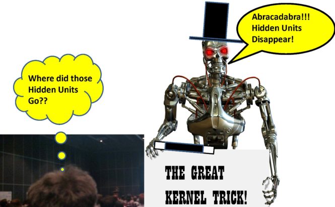
LM101-052: How to Use the Kernel Trick to Make Hidden Units Disappear

Episode Summary:

Today, we discuss a simple yet powerful idea which began popular in the machine learning literature in the 1990s which is called “The Kernel Trick”. The basic idea behind “The Kernel Trick” is that an impossible machine learning problem can be transformed into an easy machine learning problem in some cases if the training data is recoded in a particular manner. However, the storage and computation requirements involving such transformations may be excessive. The “Kernel Trick” provides a way of providing similarity relationships between the transformed training data patterns to the learning machine so that the learning machine can efficiently represent and manipulate these similarity relationships without recoding the original data set. That is, rather than specifying a “recoding transformation” for each input pattern…the basic idea of the “Kernel Trick” is that you specify similarity relationships among input patterns. In some cases, this can be advantageous while in other cases it may not be so useful.

Show Notes:

Hello everyone! Welcome to the 52nd podcast in the podcast series Learning Machines 101! In this series of podcasts my goal is to discuss important concepts of artificial intelligence and machine learning in hopefully an entertaining and educational manner.

Today, we discuss a simple yet powerful idea which began popular in the machine learning literature in the 1990s which is called “The Kernel Trick”. Typically, the “Kernel Trick” is introduced as a part of the concept of a support vector machine which was described in Episode 47 but actually the “Kernel Trick” concept is more general and is applicable to support vector machines, linear regression models, principal components analysis, and many other popular linear machine learning algorithms.

The basic idea behind “The Kernel Trick” is that an impossible machine learning problem can be transformed into an easy machine learning problem in some cases if the training data is recoded in a particular manner. However, the storage and computation requirements involving such transformations may be excessive. The “Kernel Trick” provides a way of providing similarity relationships between the transformed training data patterns to the learning machine so that the learning machine can efficiently represent and manipulate these similarity relationships without recoding the original data set. That is, rather than specifying a “recoding transformation” for each input pattern…the basic idea of the “Kernel Trick” is that you specify similarity relationships among input patterns. In some cases, this can be advantageous while in other cases it may not be so useful.

Let’s now work through a specific example and I’ll explain the above ideas in a more systematic and complete manner. Let’s start with the simplest possible example. We want to predict whether or not someone is sick by taking their temperature with a thermometer. Also assume that we have a linear machine which works by generating an output which is a weighted sum of its inputs. If that weighted sum exceeds a threshold, then the linear machine declares the person as “sick”. If the weighted sum is less than the threshold, then the linear machine declares the person as “well”.

In this case, the input pattern is a single number which is the “temperature”. Then the learning machine will classify the person as “sick” if the temperature exceeds some critical value. Ideally, the learning machine would “learn” from its experiences how to set the threshold so that if someone’s temperature was greater than 100 degrees or 101 degrees then they should be classified as “sick”. However, the problem is complicated by the fact that if you have a very low temperature then you are also sick! So if you have a temperature of less than 96 degrees you would also be “sick”! This clearly poses a problem for this type of learning machine since this problem is too “nonlinear” for a simple learning machine which classifies someone as “sick” or “not sick” by checking if the input body temperature is above some threshold value. That is, it is IMPOSSIBLE to set the threshold correctly so that the learning machine will work correctly. We encountered a similar problem with linear learning machines in Episode 14 and Episode 15 in Learning Machines 101 when we noted that a linear learning machine could not solve the exclusive-or problem.

One option is that we replace our simple learning machine with a more advanced nonlinear learning machine which decides if you are “sick” if your temperature is too low or your temperature is too high. Examples of more advanced nonlinear learning machines which do “deep learning” are described in Episode 14, Episode 15, and Episode 41. Such learning machines have multiple layers of hidden units and are capable of learning arbitrary functions. In fact, if we used a nonlinear learning machine with one layer of hidden units which took our temperature input and then projected it to a group of hidden units and then the output of the hidden units projected to the response unit we could solve this problem!

For example, we can actually solve this problem with two nonlinear hidden units. We have one sigmoidal hidden unit which “turns on” if the temperature of the person is too high. We have another sigmoidal hidden unit which “turns on” if the temperature of the person is too low. In addition, assume that if either hidden unit “turns on” then this will generate an output response above the threshold indicating the person is “sick” but if both hidden units are “off” then the generated response is below the threshold indicating the person is “well”. To summarize, a linear machine with one temperature input number and one output which indicates whether the person is sick can not solve this problem because it can not represent the solution. However, a nonlinear learning machine…specifically a nonlinear learning machine which has one input for temperature which feeds into two hidden units and then these two hidden units feed into the output can solve this problem. This type of learning machine architecture is the basic deep learning architecture discussed in Episode 14, Episode 15, and Episode 41. Note this was a very simple problem where the input pattern is one number and the relationship between the input pattern of one number and the output pattern of one number is quite simple. In a more realistic complicated situation where the person’s health is evaluated with hundreds of measures such as: temperature, blood pressure, body weight, age, exercise frequency, calories per day, body fat, and so on….if the problem is nonlinear then many hidden units or many layers of hidden units might be required to solve the problem.

So why not just solve the problem with such a nonlinear learning machine? There are two main reasons: (1) nonlinear learning machine with hidden units might take hours, days, or weeks to train, (2) the connection weights or parameters of a nonlinear learning machine can easily converge to the wrong answer so even after training the machine for weeks you may find you have to start all over because you converged to the wrong answer, and (3) it is difficult to determine if you have the right number of layers or right number of hidden units or the right type of hidden units to solve the problem.

In contrast, even though many problems are impossible for a linear learning machine to solve, if the problem can be solved by a linear learning machine, then the linear learning machine can often solve the problem on a time-scale of seconds or minutes rather than hours or days. In addition, linear learning machine algorithms are typically guaranteed to converge to the best solution. So this means that after learning, even though the final answer may not be that great for a linear learning machine, it is the best possible answer given that you used a linear learning machine.

So…as you can see…the linear and nonlinear learning machines both have advantages and disadvantages. If the problem is solvable by the linear learning machine, then the linear learning machine can solve the problem much more quickly and accurately than the nonlinear learning machine. However, there are many problems which can’t be solved by the linear learning machine. The “Kernel Trick” tries to merge the best features of both the linear and nonlinear learning machines without incorporating the bad features! This is how it works!

Let’s return to the problem of classifying someone as “sick” or “well” based upon measuring the temperature of that person with a thermometer. As we previously observed, a linear machine can not solve this problem but a nonlinear machine can solve this problem. We can visualize how the nonlinear machine solves this problem in the following manner. Essentially, the nonlinear machine “learns” how to connect input units to hidden units in just such a way so that the pattern of states over the hidden units corresponds to a “recoding transformation” of the original input pattern. In our example, a particular number corresponding to a temperature is mapped into two numbers corresponding to the hidden unit states. If the temperature is above some threshold, then the numerical temperature value is mapped into a two-dimensional hidden unit activation pattern where the first hidden unit is on and the second hidden unit is off. If the temperature is below some threshold, then the numerical temperature value is mapped into a two-dimensional hidden unit activation pattern where the first hidden unit is off and the second hidden unit is on. If we were to recode the original temperature inputs as a set of 2-dimensional patterns and then fed these binary 2-dimensional input patterns into a linear machine then the linear machine could learn to solve this problem.

There are many ways to “transform” or “recode” an input pattern so that a problem which is impossible for a linear machine to solve becomes easy for it to solve. Here is another way we can “recode” the temperature input pattern for our linear machine so that the linear machine can correctly predict whether someone is sick or well. Suppose the transformed temperature is defined according to the following rule. Take the original temperature, subtract 98.6 from the original temperature, then square that difference. With this nonlinear transformation, the learning machine might learn a threshold value of 3 (since 1.5 squared is 3) which would result in the learning machine classifying a temperature above 98.5 + 1.5=100 as “sick” or a temperature below 98.5-1.5=97 as “sick”. In other words, the learning machine computes the squared deviation of the original temperature from 98.5 and checks that the squared deviation is less than 1.5 squared.

So…this illustrates the key point. If we have a “linear learning machine” by simply changing the representation of its input patterns we can get it to solve a “nonlinear problem”. So this leads us to the next key point. Suppose we have a nonlinear learning problem and a “linear learning machine”, how do we figure out the right nonlinear transformation of the input pattern so a linear learning machine can solve our nonlinear problem? This is the type of problem that we want to focus our attention upon.

It turns out that if the response of the linear learning machine is numerical, then a commonly used linear learning machine is “linear regression” where the goal of the linear learning machine is to minimize the sum-of-squared difference between the machine’s numerical prediction and the desired numerical response. If the response of the linear learning machine is binary (e.g., a 0 or a 1), then a commonly used linear learning machine is a “support vector machine” where the goal of the linear learning machine is to minimize the number of times the linear learning machine’s predicted response which is a 0 or 1 disagrees with the desired response which is a 0 or 1. The mathematical formulas used to compute the answers in both of these cases are quite computationally efficient and answers for very large complex problems can be often obtained within seconds or even fractions of seconds. In the following discussion, we will use the terminology “linear learning machine” to refer to either or both the linear regression learning machine and the linear support vector learning machine. There are actually many other types of “linear learning machines” which are compatible with the following discussion but we won’t go into those in this brief introduction.

As previously noted, linear learning machines are computationally limited and won’t be able to solve many important nonlinear problems. Note, however, that if we had a “recoding transformation” that could map the original input pattern into a new pattern then we could train the linear learning machine with the “recoded” input patterns and if we had just the right “recoding transformation” the linear learning machine would be able to solve the nonlinear problem! As noted in Episode 14, Episode 15, and Episode 41. If we feed the input units into a set of hidden units and then feed the hidden units into the output units, then we should be able to solve any nonlinear problem if the number of hidden units is sufficiently large….taking into account that this argument ignores issues such as generalization performance and focusses upon simply learning training data.

So what we are going to do is to simply feed transformed patterns into the linear learning machine to solve the nonlinear problem. The problem is how do we pick the nonlinear transformation? One approach is to use a nonlinear learning machine so that this nonlinear transformation is learned as in Deep Learning Networks as described in Episode 14, Episode 15, and Episode 41. Another approach is to use the “Kernel Trick”.

The basic idea of the “Kernel Trick” is that if we carefully examine the mathematical formulas used to estimate the parameters and make predictions for the linear regression learning machine and the linear support vector learning machine we discover a fascinating and important fact. All of the formulas used for learning and making predictions can be written without knowing the identity of the nonlinear transformation used to code the input patterns!!!

Instead, what is required is information about dot product between every pair of transformed input patterns. The concept of a dot product was described in a previous episode of Learning Machines 101. For now, we can think of the dot product between two transformed input pattern vectors as a measure of their similarity. Thus, the collection of all such dot products can be referred to as a “Similarity Matrix”. The important and non-trivial fact is that all of the formulas for both learning and prediction using either the linear regression or the linear support vector machine in the case where nonlinear transformations are applied to the input patterns can be rewritten without explicitly knowing the nonlinear transformations!! Instead, we simply need to have a formula which lets us compute the similarity between two transformed input patterns! This formula is called a “kernel”!!

We can then specify a “kernel” and plug the kernel into formulas for linear regression learning and linear support vector learning machines. One important benefit of the “kernel” function is that suppose we needed millions of hidden units to solve a nonlinear problem. The “Kernel Trick” states that we don’t need to specify the identity of these millions of hidden units and we don’t need to specify how the input units are connected to the hidden units. All we need to specify is how to measure the “similarity” between a given pair of hidden unit patterns induced by a respective pair of input pattern vectors using our Kernel Function which takes as input two input vectors and returns a number! This can vastly simplify the computational requirements for both learning and prediction. Moreover, in many important cases, the machine learning design engineer might have good intuitions regarding how to specify the similarity structure among input patterns but might not have good intuitions regarding how to pick an appropriate recoding transformation. This is another advantage of the “Kernel Trick”!

However, there is a “technical detail”! If we specify the kernel directly without knowledge of the nonlinear transformation used to recode the input patterns, it is possible that we will pick a “kernel” which isn’t associated with a nonlinear transformation. That is, although every nonlinear transformation of input patterns generates a “kernel” formula…it is not the case that every “kernel” formula generates a nonlinear transformation of input patterns. Since our mathematical analysis of the linear learning machine is based upon the assumption of a nonlinear transformation of input patterns we need to know that transformation exists even though we don’t actually use it in order to ensure the mathematical formulas we use are correct.

There is a famous mathematical theorem called “Mercer’s Theorem” which helps us figure out these issues. The basic idea of Mercer’s Theorem is that it provides a simple method for checking if a proposed “kernel formula” relating two input patterns could be represented as the dot product of a nonlinear transformation of one of the two input patterns and that same nonlinear transformation applied to the other input pattern. I have provided some references to Mercer’s Theorem in the notes for this episode.

Here are a few examples of kernel functions. First, take two input pattern vectors, compute their dot product, and their square that number. This procedure is an example of a “polynomial kernel”. A second example is to take two input pattern vectors, compute their dot product, multiply that by a number A, then add another number B, and then compute the hyperbolic tangent of the result. This is called a “sigmoidal kernel”. The sigmoidal kernel only satisfies Mercer’s Theorem for certain choices of A and B. A third example of a kernel is the Radial Basis function kernel. In this case, we subtract two input vectors from one another, then we compute the magnitude of the difference vector squared and then divide by a negative number, then we compute the exponential of this latter quantity. The Radial Basis Function also known as the RBF or Gaussian kernel function is widely used. It is also intellectually quite interesting because it can be shown that the RBF kernel is generated by a nonlinear transformation which transforms a finite-dimensional input pattern into a pattern with an infinite number of hidden units!! There are many more kernels as well! Cesar Souza has a nice website about kernel functions for Machine Learning and you can find that link in the show notes of this episode. He mentions the: linear kernel, polynomial kernel, Gaussian Kernel, Exponential Kernel, Laplacian Kernel, ANOVA Kernel, Hyperbolic Tangent Sigmoid Kernel, Rational Quadratic Kernel, Multiquadric Kernel, Inverse Multiquadric Kernel, Circuluar Kernel, Spherical Kernel, Wave Kernel, Power Kernel, Log Kernel, Spline Kernel, B-Spline Kernel, Bessel Kerenel, Cauchy Kernel, Chi-Square Kernel, Histogram Intersection Kernel, Generalized Histogram Intersection Kernel, Generalized T-Student Kernel, Bayesian Kernel, Wavelet Kernel. Also he provides some nice tutorials, source code, and additional references!

But that’s not all! Not only do we have a lot of possible kernels to choose from but we can combine kernels to get new kernels! So for example, the product of two kernels which satisfy Mercer’s Theorem is also a kernel which satisfies Mercer’s Theorem. A polynomial with non-negative coefficients of a kernel which satisfies Mercer’s Theorem is also a kernel which satisfies Mercer’s Theorem, an exponential of a kernel is a kernel as well. Bishop in Chapters 6 and 7 of his book provides a great discussion of Kernel methods and discusses in detail rules for combining kernels as well as the specific formulas for using Kernels with linear learning machines.

To summarize, the basic idea behind “The Kernel Trick” is that an impossible machine learning problem can be transformed into an easy machine learning problem in some cases if the training data is recoded in a particular manner. However, the storage and computation requirements involving such transformations may be excessive. The “Kernel Trick” provides a way of providing similarity relationships between the transformed training data patterns to the learning machine so that the learning machine can efficiently represent and manipulate these similarity relationships without recoding the original data set. That is, rather than specifying a “recoding transformation” for each input pattern…the basic idea of the “Kernel Trick” is that you specify similarity relationships among input patterns. In some cases, this can be advantageous while in other cases it may not be so useful. Like all techniques in machine learning, we don’t want to put the Kernel Trick on a pedestal but it is a good trick to include in our Machine Learning Magic Show! A definite winner!

Thank you again for listening to this episode of Learning Machines 101! I would like to remind you also that if you are a member of the Learning Machines 101 community, please update your user profile and let me know what topics you would like me to cover in this podcast.

You can update your user profile when you receive the email newsletter by simply clicking on the: “Let us know what you want to hear” link!

If you are not a member of the Learning Machines 101 community, you can join the community by visiting our website at: www.learningmachines101.com and you will have the opportunity to update your user profile at that time. You can also post requests for specific topics or comments about the show in the Statistical Machine Learning Forum on Linked In.

From time to time, I will review the profiles of members of the Learning Machines 101 community and comments posted in the Statistical Machine Learning Forum on Linked In and do my best to talk about topics of interest to the members of this group!

And don’t forget to follow us on TWITTER. The twitter handle for Learning Machines 101 is “lm101talk”!

And finally, I noticed I have been getting some nice reviews on ITUNES. Thank you so much. Your feedback and encouragement is greatly valued!

LM101-052: How to Use the Kernel Trick to Make Hidden Units Disappear

LM101-052: How to Use the Kernel Trick to Make Hidden Units Disappear

Episode Summary:

Show Notes:

Further Reading:

Leave a Reply Cancel reply