LM101-046: How to Optimize Student Learning using Recurrent Neural Networks (Educational Technology)

Teaching students using deep knowledge tracing.

Podcast: Play in new window | Download | Embed

LM101-046: How to Optimize Student Learning using Recurrent Neural Networks (Educational Technology)

Episode Summary:

In this episode, we briefly review Item Response Theory and Bayesian Network Theory methods for the assessment and optimization of student learning and then describe a poster presented on the first day of the Neural Information Processing Systems conference in December 2015 in Montreal which describes a Recurrent Neural Network Educational Technology approach for the assessment and optimization of student learning called “Deep Knowledge Tracing”.

Show Notes:

Hello everyone! Welcome to the forty-sixth podcast in the podcast series Learning Machines 101. In this series of podcasts my goal is to discuss important concepts of artificial intelligence and machine learning in hopefully an entertaining and educational manner. In this podcast, we continue our discussions of the relevance of machine learning in the area of educational technology by discussing a poster presented at the 2015 Neural Information Processing Systems Conference in Montreal by Chris Piech and his colleagues from Stanford University titled “Deep Knowledge Tracing”.

In the field of Deep Knowledge Tracing, it is assumed that the student is interacting with a computer for the purposes of learning. The terminology “student” could be broadly defined to include grade school students, high school students, college students, graduate students, and professionals pursuing post-graduate education. The computer presents a question to the student and the student submits their answer to the question. Questions can include a variety of forms such as multiple choice, matching, and essay questions but for the purposes of this presentation it is helpful to think of a question as a multiple choice question.

In this paper, Piech and his colleagues discuss a Recurrent Neural Network as described in Episode 36 of this podcast series to make predictions regarding what questions a student will be able to answer after the student completes each exercise. That is, the recurrent network attempts to track the evolution of the student’s knowledge state in real-time. In other words, a machine learning algorithm is used to learn a student’s knowledge state and update the current assessment of the student’s knowledge state each time the student generates an answer to an assessment question. The ability to successfully make such predictions in real-time has numerous advantages.

First, this could in principle eliminate more formal testing from the classroom environment. Tests are time-consuming to administer and reduce precious classroom time which could be used for learning. One could imagine that the questions generated by the Deep Knowledge System are designed primarily to support and grow student understanding with assessment being only a secondary priority. Human instructors could devote more classroom time to explaining difficult concepts, working out solutions to problems, and answering questions.

Second, by monitoring a student’s knowledge state in real time, this would allow a real-time evaluation of gaps in student knowledge. Upon identifying the presence of a student knowledge gap, the machine learning system could generate more questions intended to grow student understanding in that area and would avoid questions designed to grow understanding in areas that they have already mastered.

In Episode 37 we discussed an important earlier approach to this problem called Item Response Theory which can be interpreted as a very simple yet powerful type of machine learning algorithm developed in the 1980s. The essential idea of Item Response Theory is that the probability that a student answers a question correctly is a function of three free parameters. It is assumed that the student can answer a question correctly by either guessing the answer with probability C or the student fails to correctly guess the answer. If the student fails to correctly guess the answer, then the probability that the student correctly answers the question is assumed to increase as a function of the difference of the student’s ability to answer questions in that knowledge domain represented by the variable A minus the difficulty of the particular question which is represented by the variable B.

For example, suppose that a group of 30 questions to be presented to the student can be divided into three groups which are designed to assess the student’s understanding of three different concepts. During the assessment process, the student would be presented with 30 questions and each question would be associated with an item difficulty parameter which presumably has already been estimated from a larger data sample. Also assume that the parameter specifying the probability of guessing has also been estimated from a larger data sample. You can probably think of several ways to improve this setup such as making the guessing parameter question-specific or student-specific but let’s consider this simplified problem for expository reasons.

Thus, for each student, one would estimate 3 parameters: three parameters for the three different concepts even though the student answers 30 questions. Even before all 30 questions are answered, the computerized testing system can assess which of the three target concepts requires the most mastery. In addition, because each question is associated with a difficulty parameter, the system can compare the student’s mastery of a concept with the difficulty of a question and attempt to present questions which are neither too easy or too difficult for the student to support an optimal learning experience for the student.

So this is an example of a more classic approach to using machine learning for the purpose of optimizing student learning experiences and assessing student knowledge in real-time.

In Episode 38, we discussed another approach to the adaptive assessment of online student learning based upon a paper recently presented by Gonzalez-Brenes presented at the 2015 International Conference on Artificial Intelligence and Statistics which was held in San Diego, California. This model was called the “Dynamic Cognitive Tracing Hidden Markov Model” which can be considered to be an example of a Bayesian Network Theory model.

In this version of a Bayesian Network Theory model, it is assumed that one begins with a fixed number of items. An item corresponds to a particular template for generating a question on an exam. It is assumed that the answer to an item is either “correct” or “incorrect”. For example, an item might be generated from a template which specifies a problem consisting of applying the Calculus chain rule to compute the derivative of a function of a function of a single variable. The responses to the problem might be multiple choice responses corresponding to different choices for the derivative. For each of a fixed number of items, it is assumed that there exists a probability distribution which specifies the probability that one of a fixed number of possible skills is relevant to the solution of the problem. Although technically this assumption means that only one skill is required to answer a particular item and the the percentage of times a skill S is required to answer the item for a particular item is equal to Ps. In spirit, however, the semantic intention of this assumption is that all skills are relevant to the solution of item I with the degree of relevance of skill S being defined by the probability Ps. This is a subtle semantic interpretation of the model but it is quite crucial for understanding the objective of the modeling process. It is based upon interpreting the probability distribution as a theory of belief as described in Episode 8 but estimating this belief distribution using frequentist concepts. In other words, given a particular item, the probability model assigns a degree of belief that a particular skill is used for that item. These degrees of belief are then estimated using frequentist assumptions.

Thus, the item-specific parameters associated with an item specify a probability distribution over the set of skills. These item-specific parameters are not functionally dependent upon the ability of a particular student but rather are common to all students in the student population. In addition, we have student-specific parameters which are different for each student. These student specific parameters specify the probability distribution the student has mastered skill S at time t given the student has mastered skill S at time t-1. It is assumed that there are different levels of mastery for each skill. For example, one might imagine there are three levels of mastery for a particular skill which are: novice, intermediate, and expert.

This means that the time-course of a student’s mastery of skills over time is represented by a collection of probability distributions which specify the probability of the skill profile of the student at time t given the skill profile of the student at time t-1. This is essentially a Markov chain as described in Episode 11. Finally, the probability that the student answers an item correctly at time t is functionally dependent upon the current skill profile which indicates which indicates the knowledge level such as “novice” or “expert” for each skill as well as the likelihood that the particular skill is relevant for answering the item presented at the current time. This is called a Bayesian network and it is a generalization of the Markov model approach. In a manner analogous to the simpler Item Response Theory approach, we thus can estimate parameters of the model which are student-specific and and parameters of the model which are item-specific.

In contrast to the Item Response Theory and the Bayesian Network Theory approaches, the RNN approach is much less structured and is driven more by statistical regularities in the data. This has some advantages in that potentially more sophisticated internal representations of student knowledge structures might be identified but more data is required and additional challenges concerned with problems of estimation and overfitting must be addressed.

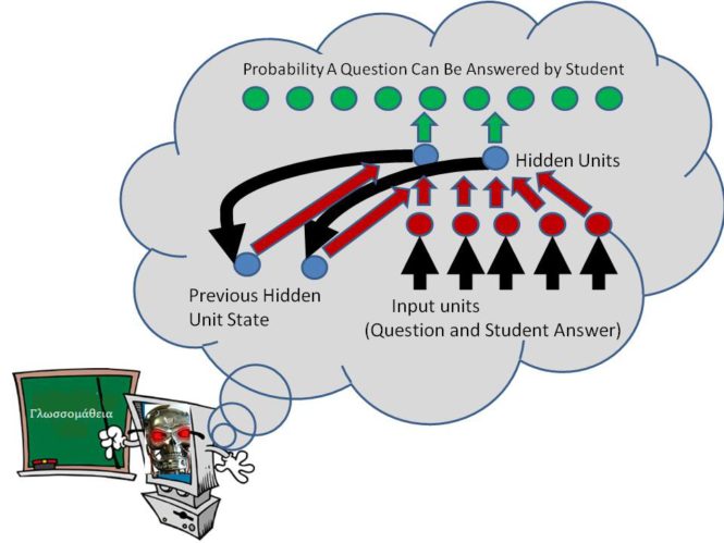
A recurrent neural network or RNN can be viewed as a mechanism which maps a sequence of input patterns into a sequence of output patterns. In this context, an input pattern of ones and zeros is used to specify which problem was answered and whether or not that problem was correctly answered. This means that for a set of 50 possible problems, then the number of elements in the input pattern could potentially be extremely large. The RNN then uses the past history of input patterns and the current input pattern to generate the output pattern for the current input pattern. For an assessment with 50 possible questions, the output pattern only contains 50 elements where a particular output element is interpreted as the probability that a particular question in the problem set is expected to be answered correctly by the student.

The details of the simplified version of the RNN are now provided. The RNN has 50 output units. Each output unit is associated with a number between 0 and 1 called the output unit’s state. An output unit’s state is interpreted as the probability that a particular question is known to the student. This output probability is computed using a sigmoidal function as defined in Episode 14 of a weighted sum of the states of a set of hidden units. Each hidden unit state is then computed using a hyperbolic tangent sigmoidal function of a weighted sum of the current input pattern plus a weighted sum of the previous hidden unit states. This recursive structure encourages the development of a compressed representation of the past history of the input patterns for predicting the current estimated probability that the student knows a particular question.

The parameters of the RNN are estimated by minimizing an objective function which attempts to match the model’s predicted probabilities with observed frequencies in the environment. More technically, it can be shown this objective function is a log-likelihood function so that the parameter estimates of the RNN are maximum likelihood estimates as described in Episode 26. The parameters are adjusted using the method of gradient descent which was described in Episode 31 of this podcast series. The software and preprocessed data has been made available by the authors of this article. A link for downloading this software and these data sets can be obtained by visiting the show notes for this episode at www.learningmachines101.com or going directly to the website: github.com/chrispiech/DeepKnowledgeTracing.

The performance of the RNN was evaluated using three types of data sets. The first data set was based upon a collection of 2,000 simulated students. An Item Response Theory model as described earlier was used to generate answers from the simulated students based upon five distinct concepts, 50 problems, and a random guess probability. For example, one can assume that a simulated student is represented by 5 parameter values corresponding to knowledge of each of the five basic concepts, the probability of the simulated student’s response is then functionally dependent upon the student’s 5 parameter values, the guessing parameter value, and the item difficulty parameter values. An additional assumption was introduced which gradually increased the appropriate concept parameter value for a student when the student encountered a related problem. The advantage of using simulated student data rather than real student data is that this greatly facilitates the process of evaluating the RNN’s performance since the mechanism of student response generation is known.The RNN performance in predicting performance using simulated data had predictive accuracies in the range of 75% to 85%.

In addition, the authors suggest an influence measure for estimating the evidence that a particular problem will be answered correctly based upon the answer to the current problem. When they used this measure to analyze the simulated student response data, they found that the influence relationships between pairs of student responses could naturally be grouped into five categories corresponding to the five concept categories originally used to generate the simulated data.

In addition, the RNN was evaluated using a sample of real human student usage interactions with the eighth grade common core curriculum from Khan academy. Khan academy (www.khanacademy.org) is an on-line learning environment. The data set included 1.4 million different exercises completed by 47,495 students across 69 different exercise types. Five-fold cross-validation as described in Episode 28 was used to evaluate performance on the Khan academy data. Again, the predictive performance was very impressive.

The Khan academy data was also analyzed for the purpose of identifying knowledge clusters consisting of pairs of core curriculum exercises. For example, the problem types of “bivariate data frequencies”, “linear models of bivariate data”, “plotting the line of best fit”, “interpreting scatter plots”, and “scatter plot construction” were mutually connected in the sense that knowledge of one of these problem types tended to predict with a high probability that knowledge of the other problem types is present.

The RNN was compared to a Bayesian Knowledge Network but the details of the network were not provided. The Bayesian Knowledge Network used was probably not as sophisticated as the version described in Episode 38 of this podcast series. The performance of the Bayesian Knowledge Network was actually quite poor and exhibited performance comparable to a baseline model were one simply uses the probability that a particular question will be correctly answered as the estimated probability. Although I greatly appreciated the contributions and work invested in this project, I would have liked to have a better understanding of the situations where the RNN would be superior and the situations where the RNN would be inferior to a Bayesian Knowledge Network of the type described in Episode 38.

To be sure, the RNN objective function for parameter estimation is extremely complex and high-dimensional. It would be interesting to see if a more constrained version of the RNN architecture or more sophisticated versions of Item Response Theory or Bayesian Knowledge Networks would show comparable performance. Possible limitations of the RNN approach are: uniqueness, robustness of the parameter estimation process, and overall complexity.

Well…this was a description of only one poster out of the 102 posters presented on the first night of the Neural Information Processing Systems conference in Montreal! I have a few more posters I want to discuss out of the 102 posters presented on the first night of the conference. After I complete those discussions, we will move to the second day of the conference!!!

I have provided in the show notes at: www.learningmachines101.com hyperlinks to all of the papers published at the Neural Information Processing Systems conference since 1987, the workshop and conference schedule for the Neural Information Processing Systems conference, and links to related episodes of Learning Machines 101!
If you are a member of the Learning Machines 101 community, please update your user profile. If you look carefully you can provide specific information about your interests on the user profile when you register for learning machines 101 or when you receive the bi-monthly Learning Machines 101 email update!

You can update your user profile when you receive the email newsletter by simply clicking on the: “Let us know what you want to hear” link!

Or if you are not a member of the Learning Machines 101 community, when you join the community by visiting our website at: www.learningmachines101.com you will have the opportunity to update your user profile at that time.

Also check out the Statistical Machine Learning Forum on LinkedIn and Twitter at “lm101talk”.
Also check us out at PINTEREST as well!

From time to time, I will review the profiles of members of the Learning Machines 101 community and do my best to talk about topics of interest to the members of this group! So please make sure to visit the website: www.learningmachines101.com and update your profile!

So thanks for your participation in today’s show! I greatly appreciate your support and interest in the show!!