Podcast: Play in new window | Download | Embed
LM101-036: How to Predict the Future from the Distant Past using Recurrent Neural Networks
Episode Summary:
In this episode, we discuss the problem of predicting the future from not only recent events but also from the distant past using Recurrent Neural Networks (RNNs). A example RNN is described which learns to label images with simple sentences. A learning machine capable of generating even simple descriptions of images such as these could be used to help the blind interpret images, provide assistance to children and adults in language acquisition, support internet search of content in images, and enhance search engine optimization websites containing unlabeled images. Both tutorial notes and advanced implementational notes for RNNs can be found in the show notes at: www.learningmachines101.com .
Show Notes:
Hello everyone! Welcome to the thirty-sixth podcast in the podcast series Learning Machines 101. In this series of podcasts my goal is to discuss important concepts of artificial intelligence and machine learning in hopefully an entertaining and educational manner.
In this episode, we discuss the problem of predicting the future from not only recent experiences but also from the more distant past. Humor in language is one example. A sequence of events sets up certain expectations in the mind of the comprehender and when those expectations are violated this can result in the perception of humor as result of the resolution of the incongruity.
For example, when I was a child I noticed that most kids would get a rubber duck to play with in the bathtub, but all my parents gave me was a toaster!
And for those of you out there who are teaching writing. Here is a helpful piece of advice you can share with your students:
A preposition is something you should never end a sentence with.
These examples illustrate that the creation of expectations and consequences of a sequence of events occurs effortlessly for human comprehenders. We are constantly making predictions about the future based upon events in the past.
In the real world, comprehension of sequences of events often takes place sequentially in time on a much larger scale. Vast amounts of information are observed over long periods of time and selected information from the past must be used to correctly interpret the present. The amount of incoming information is too large to store and even if we did store large amounts of information reaching back into the distant past, we would still have the problem of selecting the small yet crucial components of that large information storage base that are important for predictions. Furthermore, the execution of specific action sequences also involves the use of temporal constraints which must operate simultaneously over both short and long periods of times. Some actions can not be performed until other actions have been correctly executed, while other actions can be performed at any time.
One useful heuristic strategy is to focus upon the most recently experienced events. This is the approach of Markov modeling described in Episode 11. Although knowledge of recent events is often very helpful for predicting current events, knowledge of the occurrence of relevant events in the distant past may play a crucial role in the interpretation, prediction, and control of current events. One strategy for making use of such information is to simply include not only the current experiences but also the entire past history of the learning machine’s experiences as inputs to the learning machine. Unfortunately, inclusion of the entire past history of the learning machine’s experiences may impose impossible storage and computation requirements. For this reason, only strategically chosen subsets of the learning machine’s past history are often used. This is an important widely used strategy where the inputs to the learning machine at the current time might not only include the values of all sensor inputs of the learning machine at the current time but also the values of all sensor inputs at the previous time interval as well as a subset of sensor inputs at a particular time interval in the distant past.
Although this is an effective approach in many situations, there also exist many situations where it is unclear which strategically chosen subsets of the learning machine’s past history should be chosen for the purposes of interpretation, prediction, and control. Recurrent neural networks or RNNs provide a method for learning how to address this problem.
For example, consider the problem of presenting an image of a “cat sitting on a box” to an RNN. And then the goal is to train the RNN to generate a well-formed sentence describing the image. During the learning process, the learning machine is provided with the image and an example of a sentence describing the image.
The learning machine must learn not only syntactic relationships among words but must also learn semantic relationships among words as well in addition to identifying objects and concepts in the image itself. In other words, if the image consists of a cat sitting on a box, then the goal is not to generate the concepts “cat”, “sit”, and “box” or a well-formed but nonsensical sentence such as “The box sits on a cat” but rather a simple well-formed semantically-meaningful sentence such as “A cat sits on the box”. The ability to generate simple sentence descriptions of images such as these has numerous practical applications. A machine capable of generating even simple descriptions of images such as these could be used to help the blind interpret images, provide assistance to children and adults in language acquisition, support internet search of content in images, and enhance search engine optimization websites containing unlabeled images.
A recent paper published as a conference paper at the International Conference on Learning Representations in 2015 titled “Deep Captioning with Multimodal Recurrent Neural Networks” describes current progress on exploring the problem of learning to generate captions for images. References to this paper and the Multimodal-RNN project website can be found in the show notes at: www.learningmachines101.com . The system was trained and tested with several data sets. For example, one of the data sets which was used is called the COCO data set which consists of 82,783 images for the training data set and an additional 40,504 images for the test data set. For each image, five different sentence captions are provided. The resulting system is competitive with other state-of-the-art systems using similar techniques by a variety of metrics and exhibits impressive performance yet does not approach human performance levels. The system works by generating the first word of a sentence given the image. Then second word of the sentence is generated from a representation of the first word
Here are a few examples illustrating the performance of the system. I’ve taken these examples from the UCLA Multimodal-RNN project website and I have provided the link to this website in the show notes at: www.learningmachines101.com . I will first describe the image using my own words and then I will provide the description provided by the RNN which was trained on the COCO dataset.
Imagine an image of a ski slope which has some trams carrying skiiers in the background. In the foreground, you see a man in a yellow jacket flying through the air above the snow on a snowboard. The computer generated caption reads:
“a man riding a snowboard down a snow covered slope”.
Imagine an image of two open boxes of pizza sitting side by side. The pizza in each box has a missing slice of pizza. Also the box on the left has some packets of parmesan cheese.The computer generated caption reads: “a pizza sitting on top of a table next to a box of pizza”.
Imagine a picture of a green leafy tree whose leaves pretty much cover the entire image
except for about 1/8 of the bottom of the image is some dirt which is hard to see because
of the shade generated by the leaves. In the center of the image located in the lower 1/8
of the image is a red fire hydrant which is very hard to see because it is in the shade and
covered by green leaves. The computer generated caption reads: “a red fire hydrant sitting in the middle of a forest”
Now that we have discussed three successful examples, let’s now discuss some example failures of the system. Considering the complexity of the problem, in my opinion these “failures” should still be considered to be successes in some sense but they are failures in the sense they do not compete with human performance.
Imagine a picture of carrots and perhaps onions in a pile on the table. The computer generated caption reads: “a bunch of oranges are on a table.”
Imagine a picture of a foot on a skateboard. The computer generated caption reads:
“a person is holding a skateboard on a street”.
Imagine four zebra against a concrete wall on a path covered by stones. The zebra are probably in a zoo. The computer generated caption reads:
“a zebra standing on a dirt road next to a tree.”
Before describing the network architecture that was used to implement the caption generating learning machine which was just described, some concepts of feedforward networks will be reviewed, followed by a quick review of the simple recurrent network or Elman network which was introduced in the 1990s.
In Episode 23, we discussed the concept of a feedforward network architecture where input signals are represented as an input pattern vector, and then each member of a set of hidden units computes a sigmoidal transformation of a weighted sum of the elements of the input pattern vector. A sigmoidal transformation means that if the hidden unit’s weighted sum is a large positive number then the hidden unit’s state is close to one, while if the hidden unit’s weighted sum is a large negative number then the hidden unit’s state is close to zero. The output of the hidden unit is approximately equal to the weighted sum of its inputs for cases where the weighted sum is close to zero. If the output of such a network is categorical which means that the desired response is exactly one choice out of M possible choices, then the output units are typically chosen to be softmax output units whose states can be interpreted as probabilities. Specifically, the states of all output units are constrained to be positive and add to one so that the kth output units may be interpreted as the probability that the desired response is the kth value of a categorical variable with M possible values. The prediction error for this type of network is designed to find the weights or equivalently parameters which maximize the likelihood of the observed data. The likelihood of the observed data is called the prediction error function.
The learning process used is typically related to a gradient descent procedure of the type discussed in Episode 16. The derivative of the prediction error function with respect to the network’s parameters is first computed. This derivative is then used to derive a gradient descent type learning rule which is defined as follows. The new parameter values are equal to the old parameter values plus a small number called the learning rate multiplied by the negative of the derivative of the prediction error function. As discussed in Episode 16, this type of procedure can be shown to decrease the prediction error. More technically, this type of feedforward network architecture can be interpreted as a nonlinear multinomial logit regression model whose parameters are estimated using maximum likelihood estimation.
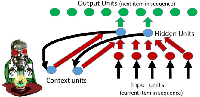
The basic Elman recurrent network originally developed in the 1990s can now be described in the following manner for learning sequences of words. An input pattern vector consisting of a list of numbers is used to represent a particular word. Each member of a set of hidden units computes a sigmoidal transformation of a weighted sum of the elements of the input pattern word vector and the elements of another vector which is called the context vector. The output units are softmax units which compute a weighted sum of the outputs of the hidden units. So this sounds pretty much the same as the description of the feedforward network architecture we previously described but there is a crucial and fundamental difference!! We explain this for an example where the Elman recurrent network is learning a 10 word sentence.
When the first word of a sentence is presented the hidden units compute a weighted sum of the elements of the input pattern representing the first word to generate a hidden unit response vector. The softmax output units then compute a weighted sum of the elements of the hidden unit response vector and generate output probabilities indicating the predicted probability of the second word in the sentence. When the second word in the sentence is presented, the hidden units compute a weighted sum the elements of the input pattern representing the second word and the elements of the context vector. The context vector is defined as the hidden unit response vector generated when the first word of the sentence was presented. When the third word in the sentence is presented, the hidden units compute a weighted sum of the elements of the input pattern vector and the elements of the hidden unit response vector generated when the second word in the sentence was presented. But the hidden unit response vector generated when the second word in the sentence was presented was functionally dependent upon the first two words! It follows therefore that the context vector contains a representation of past history of words that were presented to the system. Moreover, this is a compressed representation which doesn’t include all possible information but rather just those properties of the past history which were relevant for making predictions about the next word in the sentence!
It is important to understand how the learning process in an Elman RNN differs from the feedforward network architecture. Although the process is exactly the gradient descent method described in Episode 16, one must be careful to compute the derivative of the prediction error correctly. The derivative of the prediction error for the Elman RNN is not the same as the derivative of the prediction error for the feedforward network. Intuitively, the gradient descent learning algorithm for an Elman RNN works as follows. After presenting the Elman RNN with a sequence of words, one obtains a prediction error for the output of the RNN
for each word in the sequence. The prediction error for the hidden units for a particular word in the sequence is computed not only from the prediction error of the output of the RNN as in the standard feedforward network but also depends on the prediction error for the hidden units for the subsequent word in the sequence. This more complex calculation of prediction errors directly follows from computing the derivative of the Elman RNN prediction error. Once the prediction errors for the output units and hidden units for a sentence have been computed, then the parameter value or connection weight from unit A in the network to unit B is computed by perturbing that connection weight by an amount directly proportional to the prediction error for unit B multiplied by the state of unit A.
As a consequence of this type of learning procedure, one sometimes encounters what is called the vanishing and exploding gradient problem which is discussed in a recent paper by Pascanu et al. If the learning rate is too small, then the progressive multiplication of prediction errors for a recurrent network with many layers tends to make the prediction error vanishingly small. While if the learning rate is too large, then the progressive multiplication of prediction errors for a recurrent network with many layers might tend to make the parameter values explode.
At this point, the basic structure of the multimodal Recurrent Neural Network (m-RNN) used to obtain the results previously reported here is described. In this discussion, I will just give a simplified presentation of the approach, please see the paper in the show notes for the more technical details. The multimodal RNN works as follows. The output layer of the m-RNN is a set of softmax units where each unit corresponds to the probability that a particular word will be the next word in the sentence. Feeding into the output softmax layer is the multi-modal layer which computes a hyperbolic tangent sigmoidal function of a weighted sum of its inputs. The inputs to the multi-modal layer consist of a weighted sum of the current word pattern vector in the sentence plus a weighted sum of the context pattern vector plus a weighted sum of high-level image features. The high-level image features were derived by using a convolutional neural network with multiple layers to learn high-level features in the image corresponding to objects or object properties. This part of the network is fixed and not learnable but it was originally obtained by a learning network strategy such as described in Episode 29. The context pattern vector is computed by applying a rectified linear nonlinear transformation as described in Episode 29 of a weighted sum of the hidden unit response to the previous word plus the current word pattern vector. The rectified linear unit transformation seemed to play an important role in dealing with the vanishing and exploding gradient problem in this context. In a footnote in the paper, they noted that when the authors tried using the sigmoidal and hyperbolic tangent transformations rather than the rectilinear transformation, an exploding gradient problem was observed with the learning algorithm.
Other methods for dealing with the exploding gradient problem involve the use of normalized gradient descent where one divides the gradient by its magnitude or its magnitude over the recent history. This approach is related to the ADAGRAD method. Another way of normalizing the gradient is to use the sign of the gradient rather than its numerical values. This is related to an approach called RPROP. A review of some of these methods and related methods may be found in the article titled “Adaptive Subgradient Methods for Online Learning and Stochastic Optimization” whose hyperlink is in the shownotes at: www.learningmachines101.com . I have also provided some blog dicussions on ADAGRAD and RPROP which are a little easier to read. An extremely important approach to learning in recurrent networks is the LSTM method which essentially teaches the network to learn from experience how to weight the relevant importance of the current input and the context unit contributions. I have provided some references to the LSTM method in the show notes as well. I have included both references which are highly intuitive without any mathematics as well as references which have the explicit mathematics to support implementation and mathematical analysis.
All of these methods ADAGRAD and RPROP which essentially keep the gradient direction from getting too small or too big by normalization or LSTM which is a more sophisticated approach or SOFTPLUS and RECTILINEAR units are important tools for dealing with the vanishing and exploding gradient problem in recurrent networks!
And speaking of exploding, before all of our brains explode, I think it would be prudent to end this episode of Learning Machines 101 at this point!!!
So thanks for your participation in today’s show! I greatly appreciate your support and interest in the show!!
If you are a member of the Learning Machines 101 community, please update your user profile. If you look carefully you can provide specific information about your interests on the user profile when you register for learning machines 101 or when you receive the bi-monthly Learning Machines 101 email update!
You can update your user profile when you receive the email newsletter by simply clicking on the:
“Let us know what you want to hear” link!
Or if you are not a member of the Learning Machines 101 community, when you join the community by visiting our website at: www.learningmachines101.com you will have the opportunity to update your user profile at that time.
Also check out the Statistical Machine Learning Forum on LinkedIn and Twitter at “lm101talk”.
From time to time, I will review the profiles of members of the Learning Machines 101 community and do my best to talk about topics of interest to the members of this group!
Further Reading:
Understanding LSTM Networks (Colah’s Blog), August 27, 2015.
A good intuitive discussion of LSTM networks without the math.
The Unreasonable Effectiveness of Recurrent Neural Networks (Andrej Karpathy Blog, 2015).
Another good intuitive discussion of LSTM networks without math but a little more technical and good review of applications. Cool computer demos!!!
Speech Recognition with Deep Recurrent Neural Networks (Graves, Mohammed, and Hinton, 2013). Mathematics of LSTM networks is clearly presented.
Long Short-Term Memory Recurrent Neural Network Architectures for Large Scale Acoustic Modeling. Sak, Senior, Beaufays (Interspeech, 2014).
Mathematics of LSTM networks is clearly presented.
ADAGRAD Blog Entry (2014). Some example code. Good discussion!
RPROP paper (1994). Classic paper on RPROP.
Deep captioning and multimodal recurrent networks (source of information for podcast!)
Multimodal-RNN project website (source of information for this podcast!!!)
Vanishing and Exploding Gradient Problem. Pascanu et al. also see classic paper by Hochreiter and Schmidhuber
Elman (1991). Simple Recurrent Network. Machine Learning Paper.
Related Episodes of Learning Machines 101:
Episode 11 (Markov Modeling), Episode 16 (Gradient Descent), Episode 23 (deep learning and feedforward networks), and
Episode 29 (Convolutional Neural Networks and Rectilinear Units).
