LM101-023: How to Build a Deep Learning Machine (Function Approximation)

Robot learning to play checkers using deep learning.

Podcast: Play in new window | Download | Embed

Episode Summary:

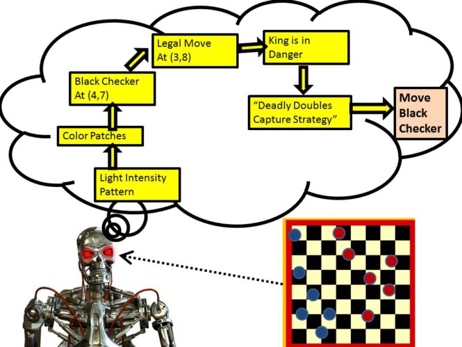
In this episode we discuss how to design and build “Deep Learning Machines” which can autonomously discover useful ways to represent knowledge of the world.

Show Notes:

Hello everyone! Welcome to the twenty-third podcast in the podcast series Learning Machines 101. In this series of podcasts my goal is to discuss important concepts of artificial intelligence and machine learning in hopefully an entertaining and educational manner.

Recently, there has been a lot of discussion and controversy over the hot topic of “deep learning”. Deep Learning technology has made real and important fundamental contributions to the development of machine learning algorithms in a variety of areas including: speech recognition, signal processing, music recognition, Google image search, figuring out the meanings of words, identifying AMAZON customer reviews as either supportive or unsupportive, understanding video clips, translating from one language to another in real time, identifying new molecules to create new advanced drugs, and help driverless cars interpret and understand complex traffic environments. A recent TED Talk by Jeremy Howard discusses some of the great achievements of Deep Learning. The talk is titled: “The Wonderful and Terrifying Implications of Computers That Can Learn”. If you visit the website: www.learningmachines101.com you can find the link to this TED Talk video.

In an article published in the April 23, 2013 edition of MIT Technology Review, Deep Learning was described as one of the top 10 Breakthrough Technologies in 2013. The idea of deep learning is described in the article as a way to make “artificial intelligence smart” and as a way to learn to recognize patterns in the world using an “artificial neural network”. Professor Hinton a leader and pioneer in the field of Deep Learning was hired on a part-time basis several years ago to lead efforts in the development of Deep Learning Technology for Google. Professor Hinton’s contributions to Google’s technology development efforts are discussed in a January 2014 article published in Wired magazine “Meet the Man Google Hired to Make AI a Reality”. The article describes the concept of “deep learning” as a “purer form of artificial intelligence” which is based upon the idea of trying to “mimic the brain using computer hardware and software”.

Other companies have also recently hopped on the Deep Learning bandwagon. Professor Yann Le Cun, another pioneer and leader in the field of Deep Learning, now works part-time at Facebook to develop Deep Learning Technology. The Forbes Website reported last year that Stanford University Professor Vincent Ng, a third leader in the field of Deep Learning, is now working part-time at the Chinese Search Engine company Baidu in order to assist in the development of Deep Learning Technology as well.

If you visit the website: www.learningmachines101.com you can find some links to interviews with Professor Hinton, Professor Le Cun, and Professor Jordan on the topic of “Deep Learning”.

So what exactly is Deep Learning Technology? Well, the first thing to understand is that Deep Learning Technology is more of a philosophical approach to developing smart learning machines rather than a specific module which you download and install into your computer to turbo charge your existing artificial intelligence modules. Most researchers in the field of Artificial Intelligence will agree that the representation of a problem in artificial intelligence is fundamentally important to obtaining a solution to that problem. How knowledge is represented and how information is represented for a machine learning algorithm can determine whether or not a particular problem’s solution is either easy or impossible.

Traditionally, the representation of a problem has always been considered a component of the engineering design process. The artificial intelligence engineer uses his or her expertise to construct a set of features that can adequately represent the statistical environment within which the learning machine lives. Even for unsupervised learning problems, considerable effort is often expended in the design and development of methods for representing the world as lists of features. For example, suppose that that you had a learning machine which was doing either supervised or unsupervised learning within its environment. The purpose of the learning machine is to learn about weather patterns. Some of the features that will be observed by the learning machine are numerical such as today’s temperature or today’s humidity level, while other features might be more categorical such as is today a “sunny day” or is it a “rainy day”. There might be thousands of features that could be collected and fed into such a learning machine. For each of these features, one needs to make decisions about how the inputs should be represented for the learning machine.

For example, should temperature be represented as a number on the Fahrenheit scale where human body temperature is 98.6? Or should it be represented as a number on the Celsius scale where human body temperature is 37? Or should it be represented as a number on the Kelvin scale where human body temperature is 310.1? Or should we represent temperature as a normalized number where we take the temperature on the Farenheit Scale and divide by 100 so that a temperature of 100 degrees Farenheit is represented as the number 1 and a temperature of 80 degrees Farenheit is represented as the number 0.8?

Or should temperature be represented as one of the following categories: “Very Cold”, “Cold”, “Warm”, “Hot”, and “Very Hot”? If so, then how should category data be represented numerically? We could represent “Very Cold” as 1, “Cold” as 2, “Warm” as 3, “Hot” as 4, “Very Hot” as 5? Or would it be better to represent “Very Cold” as -2, “Cold” as -1, “Warm” as 0, “Hot” as 1, and “Very Hot” as 2. Or we could use 5 different numbers to represent the different categories so that “Very Cold” is represented by having the first number be equal to 1 and the other 4 numbers are zeros. In other words, “Very Cold” would be represented by the list of numbers: 1,0,0,0,0. Similarly, the category “Cold” would be the list of numbers: 0,1,0,0,0; “Warm” would be the list of numbers: 0,0,1,0,0; “Hot” would be the list of numbers: 0,0,0,1,0, and “Very Hot” would be the list of numbers: 0,0,0,0,1.

One might think such discussions are not very helpful since there are so many ways the same information can be represented. However, it is a fact of life that the same learning machine will exhibit dramatically different performance depending upon how the same information is represented. If information is represented correctly, the learning machine might learn at an incredible rate and exhibit brilliant inferences and generalization performance. If information is represented incorrectly, the learning machine might find the exact same problem represented in a different way to be absolutely impossible to learn. These issues of representation are discussed in greater detail in Episode 15 of this podcast series.

Traditionally, the artificial intelligence expert has a good understanding of the problem a learning machine is supposed to solve as well as the types of data representations that are most appropriate for training that learning machine. The expert then “hand codes” the features. This is an essential part of the problem of designing an artificially intelligent system. Another aspect of the feature representation design process is that the expert must determine which features should be used to represent the statistical environment of the learning machine. As previously noted, there might be thousands and thousands of possible features that could be used to represent the learning machine’s environment but the performance of the learning machine will generally dramatically improve if the number of features is relatively small and the features are not extremely “redundant”.

Consider the following “redundant feature” problem. Suppose we are trying to predict the stock market. Our goal is to predict whether a security’s price will go “up” or go “down”. We have one feature which specifies the recent historical trend for that security and other features specifying the recent historical trends for hundreds of other features. By historical trend, I mean a few numbers which indicate whether the security’s price changes over the recent time period is upward, downward, or remaining relatively constant.

So this is a supervised learning problem where we are trying to predict whether a security’s price will go up or down based upon information from many other securities. There is a lot of redundant information in this case and also a lot of ambiguity so it is quite possible the learning machine’s performance on this task would be worse if we used hundreds of securities rather than a very small number of securities to support prediction. In order to make improved predictions, we might try to predict whether or not a security’s price will go “up” or go “down” based only on two features: (1) the recent historical trend for the target security, and (2) the recent historical trend for a DOW index fund. Most learning machines would learn more effectively with only two features in this type of scenario relative to the scenario where one has hundreds or thousands of possibly redundant features. We have used our prior knowledge of how the stock market works to design a predictive model. Our philosophy is that the past history of the specific security that we are trying to predict is important but its also important to provide the learning machine with information about the behavior of the entire stock market. This latter information, however, can be summarized by just providing the learning machine with a single DOW index fund rather than the past history of hundreds of securities. If we provided the learning machine with the past history of hundreds of securities, then the learning problem for the learning machine is more complicated because it has to figure out the relative importance of hundreds of securities. If we just provide the learning machine with two securities, it just has to figure out the relative weighting of two securities. So the key point is that if those two securities are sufficient to provide the learning machine with all of the information it needs to make predictions, then the learning machine will learn faster and more efficiently if we just use two securities rather than hundreds of securities to teach the learning machine.

Another way of thinking about this is suppose we are trying to teach a human being to solve the stock market prediction task. If we tell the human being to “focus” upon just the target security and its recent behavior in the past few weeks and the performance of the DOW index and its recent behavior in the past few weeks, we might be able to quickly train the human being to make good predictions about whether a security will go up or down in price. But if we simply provide the human being with the past several weeks of security prices from the New York Stock Exchange and say “study these newspapers” and then make a prediction about whether IBM stock will go up or down”. Clearly this is a much harder learning problem. The “focusing of attention” upon the correct predictive details of the problem can potentially transform an impossibly complex learning problem into a very easy and straightforward learning problem. Just like biological human learning machines, artificially intelligent learning machines benefit from this “focusing of attention” upon the correct predictive details of the problem as well. This is the fundamental foundation of all artificial intelligence: Obtaining the correct representational assumptions or equivalently finding the right “features” to represent the environment.

So, to summarize, machine learning problems can be solved more effectively if we have the right types of features for representing the information that the learning machine is supposed to learn. It’s also important that we have a relatively small set of features which is not redundant and identifies the key features of the environment which need to be learned. So, not only do these critical features need to be selected from an enormously large list of possible features, the method for representing each feature as either a SINGLE number or a COLLECTION of numbers must be chosen. The problem of feature selection and feature representation is of fundamental importance.

The essential goal of most Deep Learning methods is to learn a useful set of features for representing the learning machine’s environment for the purpose of facilitating learning and generalization performance by the learning machine. Deep learning methods tend to focus on learning machines which have multiple layers of processing units. So, for example, the inputs to the system are processed by the “input units”. The features for the input units are chosen by the artificial intelligence engineer. Then the outputs of the “input units” are fed into the inputs of the first layer of “hidden units”. Then the outputs of the first layer of “hidden units” are fed into the inputs of the second layer of “hidden units”. Then the outputs of the second layer of “hidden units” are fed into the inputs of the third layer of “hidden units”. Then the outputs of the third layer of “hidden units” are fed into the fourth layer of “hidden units”. This process continues until the final layer of hidden units is reached. At this point the output of the final layer of hidden units is used to make a prediction if the learning machine is a supervised learning machine. Perhaps the earliest Deep Learning Architecture was the Neocognitron which proposed by Professor Fukushima in the 1980s as a hierarchical multi-layer network for visual pattern recognition inspired by the architecture of the brain. But one could also consider the original Perceptron proposed in the late 1950s as an example of a Deep Learning architecture as well although the features were randomly chosen in the original Perceptron architecture rather than learned.

Referring to Episode 14 titled “How to Build a Machine that Can Do Anything”, one might question why so many layers of hidden units are required. The main point of Episode 14 was that with a single layer of hidden units in many cases, any arbitrary function can be approximated to any degree of accuracy if you have enough hidden units. But if you listen again to Episode 14 you will find some comments at the end of that episode which emphasize that just because a machine can represent (or even learn) any arbitrary function with just one layer of hidden units that does not mean that you always want to limit yourself to one layer of hidden units. First, it might be the case in some situations that having multiple layers of hidden units tends to simplify the problem of learning complex statistical environments. Second, these theoretical results are based upon “memorization” rather than “generalization”. These theoretical results state that given enough hidden units, the learning machine can represent any arbitrary function but these theoretical results don’t say anything about the ability of the learning machine to generalize from experience given test stimuli which are not in the training data set. Deep learning which involves multiple layers of units is specifically designed to facilitate efficient learning in complex statistical environments while using techniques that focus on generalization rather than memorization performance.

So given a multi-layer Deep Learning network architecture, how can we design learning algorithms to train such architectures? Bengio, Courville, and Vincent (2014) use the terminology “greedy layerwise unsupervised pretraining” for referring to a class of commonly used Deep Learning techniques. We will just review two examples of the concept “greedy layerwise unsupervised pretraining”.

The first approach is based upon the Gradient Descent methods approach for multi-layer networks discussed in Episode 16. In that episode we showed how to train a network with one layer of hidden units to make predictions. We can apply this approach to a learning problem by first training a learning machine with one layer of hidden units to take the pattern of inputs and learn to predict that same pattern of inputs. If the number of hidden units is large, then the learning problem is easy. The learning machine just needs to copy the input pattern to the output units. However, if the number of hidden units is relatively small, then an informational bottleneck exists. In this latter case, the learning machine must learn a mapping from the input units to the hidden units which does not throw away too much relevant information so that it is possible to also learn a mapping from the hidden units to the output units which approximately reconstructs the original pattern over the input units. This type of learning machine is sometimes called an “auto-encoder”.

Suppose the learning machine which represents the original pattern over many units (e.g., 100,000 units), learns to map that pattern into a smaller pattern over a small number of hidden units (e.g., 100 units) and then learns to map that smaller pattern over the 100 hidden units into a larger pattern over 100,000 units which is similar to the original pattern over the 100,000 inputs. In such a situation, the learning machine has acquired a “compressed representation” of the original pattern over the 100 hidden units. In fact, this procedure (under certain conditions) is mathematically equivalent to areas of mathematics which are called “factor analysis” or “principal components analysis” when the hidden units are linear. However, nonlinear units are just as important as linear units in Deep Learning Strategies.

Ok…so now we have obtained a “compressed representation” of the 100,000-dimensional input pattern which is represented as a pattern over 100 hidden units. The next step is to use the input to hidden unit processing transformation that has been learned as a preprocessing transformation of new input patterns. After learning, the connections from the input units to hidden units are fixed and not permitted to be changed. Thus, each 100,000-dimensional input pattern is transformed into a 100-dimensional input pattern. These 100-dimensional input patterns are then fed into a second unsupervised learning network of the same type which has only 10 hidden units so that a preprocessing transformation which maps the 100-dimensional input patterns into 10-dimensional input patterns is obtained. Thus, the resulting pattern over the second group of 10 hidden units correspond to “features” extracted from the pattern of information over the first group of 100 hidden units. The pattern of information over the second group of 10 hidden units is then used to make predictions. At the end of this process, one has a multi-layer network with 100,000 input units, the first layer of 100 hidden units, the second layer of 10 hidden units, and the final layer of output units. This is the first example of a greedy layerwise unsupervised pretraining strategy.

To improve performance further, after this process is completed one can allow the parameters of all layers of the units to be adjustable and adjust all of the parameters of all layers of this multi-layer learning machine simultaneously using the Gradient Descent method provided that the “initial guess” for the parameter values is obtained using the greedy layerwise unsupervised pretraining strategy. One might wonder why is the greedy layerwise unsupervised pretraining strategy necessary? Why don’t we just define a multi-layer network originally and train it with gradient descent? The reason why is that we don’t have good “initial guesses” for the parameter values and it turns out that for many multi-layer networks without those good “initial guesses”, convergence to good solutions may take a very long time and may in some cases not even be possible.

A second approach using the greedy layerwise unsupervised pretraining strategy involves using the unsupervised learning strategy described in the previous Episode 22. One trains a network of the type described in Episode 22 with a collection of variables which are always unobservable. These unobservable variables are called the “hidden units”. In addition, the network architecture is constrained in two specific ways. First, no input unit is directly connected to any other input unit. And second, no hidden unit is directly connected to any other hidden unit. All connections are symmetric. The resulting architecture was originally proposed by Smolensky (1986) as Harmony theory and more recently has become more well-known as the Restricted Boltzmann machine. In the Restricted Boltzmann machine, the input units project a pattern to the hidden units which project that pattern back to the input units. A method for training this network using a greedy layerwise unsupervised strategy is provided by Hinton, Osindero, and Teh (2006) also see Salakhutdinov and Hinton (2009). The basic idea is that you start with a multi-layer network obtained by constraining connections in the network described in Episode 22 to the values of zero. Then you constrain the connections between all layers of the network such that the pattern of connectivity between every pair of layers is exactly the same. The parameters specifying the pattern of connectivity between a pair of layers of units is then learned which implies the connectivity pattern between all layers of units are learned. Then the pattern of connection between the input units and the first layer of hidden units is fixed so that it is not modifiable. The learning process is then repeated. Then the pattern of connections between the first layer of hidden units and the second layer of hidden units is fixed so it is not modifiable. The learning process is then repeated.

We now illustrate the general philosophy of Deep Learning with two examples. In our first example, let’s consider the Stock Market Prediction Problem. How would Deep Learning work in this context? Well, one idea might be that one might take random samples of different time periods of different lengths and use an unsupervised learning machine to look for commonly occurring patterns at a variety of different time-scales. For example, one pattern the unsupervised learning machine might discover is an “upward trend”, another pattern might be a “downward trend”, another pattern might be “no change in the securities value over that time period”. Then the past history of security prices might be represented by these features discovered by the learning machine. These features, in turn, might be presented to another unsupervised learning machine which might discover “higher-order” patterns such as: “downward trend” followed by “upward trend” or “multiple downward trends following one another”. The prediction of whether a security goes up or down is then learned by a supervised learning machine which bases its predictions upon the “higher-order” patterns.

In our second example of an image-based Deep Learning Machines, the Deep Learning Machine might be presented with bit-map images from weather satellites where each feature corresponds to just a single pixel in the image which can take on one of 256 grey-level values. A single image might consist of 100,000 pixels corresponding to 100,000 features. After the unsupervised learning machine processes images represented in terms of these Elementary 100,000 features, the machine discovers 1,000 useful “higher-order” features (e.g., short line segments, short curves, small regions of the image which correspond to filled in black circles, other small regions of the image which correspond to filled in black squares, and so on). The learning machine “discovers” these features since they are common occurrences in the statistical image environment within which it lives.

These 1000 “higher-order” features correspond to a “recoding” of the original 100,000 pixel image as a list of 1,000 numbers. So now the image represented as 1000 features is then presented to a SECOND unsupervised learning machine which figures out how to represent these images using only 20 features! These 20 features might be interpretable as evidence for “wind turbulence”, “locations of extreme heat”, “locations of extreme cold”, “snowy areas”, “rainy areas”, and so on. The output of this second unsupervised learning machine is then used to predict tomorrow’s weather. This is the essential idea of Deep Learning algorithms. The Deep Learning Machines use multiple levels of analysis to learn useful featural representations of the environment to support learning.

Another important technique used in Deep Learning System Design is a technique called “convolutional coding” or “weight sharing” in which “features” which are discovered in one part of the image are assumed to be potentially present in parts of the image where they have never occurred. This can be implemented by having the learning machine “scan” the image during the feature discovery process. If the learning machine discovers useful predictive features during the scanning process in the upper part of the image rather than the lower part of the image and then in the future that predictive feature occurs in the lower part of the image, that feature is instantly identified by the learning machine since the mechanism used to detect features in the upper part of the image is exactly the same as the mechanism used to detect features in the lower part of the image. Another way of implementing “convolutional coding” without scanning the image is to have feature detectors which are position-specific but modify the learning rule for the feature detectors so that if the parameters of one position-specific feature detector are adjusted to learn a pattern, then the parameters all other position-specific feature detectors are adjusted to learn that same pattern even though that pattern did not occur in the other locations in the image. The concept of “convolutional coding” or “weight sharing” can be viewed as a generalization of the Markov modeling assumption introduced in Episode 11. Specifically the likelihood that a feature is present at a particular point in the image is functionally dependent upon whether or not certain features are present in the neighborhood of that feature. And the parameters of this single probabilistic rule used to make these calculations is adjusted based upon data collected throughout the image during the learning process. Moreover, this single probabilistic rule is applied throughout the image during the inference process.

Note that the convolutional or weight-sharing or Markov modeling approach is not limited to image processing, one could use this approach (for example) in the Stock Market Prediction Problem. In this case, one might assume that features which correspond to market behavior discovered in one time period for one security might be very useful for characterizing the behavior of a totally different security in a totally different time period.

The idea of Deep Learning is an important advancement in the field of machine learning but it is just one of many important advancements in the field of machine learning. Unfortunately, the media has a tendency to simplify and popularize such scientific advancements. It is worrisome that Deep Learning is often described as an approach which is based upon how learning in real brains work. I would say that Deep Learning is rather, inspired by speculations regarding how learning in real brains work. But I would say the exact same thing about linear regression analysis or matrix times vector multiplication which are standard topics in statistics and linear algebra.

For example, estimating the parameters of a linear regression model can be interpreted as calculating the synaptic transmission coefficients for a highly abstract linear model of either neuronal firing rates or ionic current flow through dendritic trees. A matrix by vector multiplication can be interpreted as a highly abstract linear model of the firing rate response of a pool of linear approximations to neurons from a second group of neuronal units. And, no one would argue that matrix by vector multiplication and linear regression are fundamentally important in all areas of science, math, and engineering!

As another example, many Deep Learning proponents are fascinated with the question about learning without using a lot of prior knowledge which is definitely a great question. However, this is certainly not a feature of learning that is present in brains which use lots of prior knowledge.

I would claim that “Deep Learning” is no more or no less inspired by our understanding of the brain as a matrix by vector multiplication operation is inspired by our understanding of the brain. For we can certainly model, the response properties of neural activity using linear systems.

I am also not advocating that we should not use our knowledge of neuroscience and behavioral psychology as inspiration and guidance in the development of advanced learning machines. But just because we can model some aspects of the brain using linear systems theory doesn’t imply that any machine based upon linear systems theory processes and learns information like biological brains.

I will now like to share with you three quotes. The first quote:

“Deep-learning software attempts to mimic the activity in layers of neurons in the neocortex, the wrinkly 80 percent of the brain where thinking occurs. The software learns, in a very real sense, to recognize patterns in digital representations of sounds, images, and other data.” MIT Technology Review (2013)

And here is a second quote:
“It uses [a system] patterned…after the human brain…only one more step of development, a difficult step, is needed for the device to hear speech in one language and then reproduce it either in writing or verbally in another language” [Science, News Letter, July 19, 1958]

And here is a third quote:
“RADC became strongly convinced that developments in self-organizing systems could represent a significant breakthrough in the field of intelligent data processing…the machine [is] based on theoretical models consistent with current anatomical and physiological data” [Science News Letter, July 2, 1960]

The first quote appeared relatively recently in an article published in the MIT Technology Review in 2013 describing the concept of “Deep Learning” artificial neural nets. The second and third quotes were published respectively in the years 1958 and 1960 describing the concept of the “perceptron” neural net. In my opinion, both “Deep Learning” and the “Perceptron” represent equally important advances in the field of machine learning. However, it is important to emphasize that within a decade after the quotes describing the Perceptron Neural Network research were published, research funding and interest in the Perceptron essentially vanished. This undoubtedly was due to a large number of factors but some of these factors were simply that the “Perceptron” research was “oversold”. Episode 15 of this podcast series describes the Perceptron Neural Network in greater detail as well as providing some additional historical details of the overselling of the Perceptron.

Like Deep Learning, the Perceptron was and is a great idea. Indeed, many important machine learning algorithms today use Perceptron type architectures. The “support vector machine” and “maximal marginal classifiers” can be viewed as examples of Perceptron architectures although methods for parameter estimation and computational resources have advanced since the early 1960s. The Perceptron Learning Rule is closely related to the Widrow-Hoff or LMS learning rule and the Kalman Filter which form the foundations of modern adaptive signal processing theory. Still, despite the fact the Perceptron was a great idea, it received a wave of negative publicity possibly as a consequence of the wave of positive supportive publicity it received in the late 1950s and early 1960s.

The same thing happened in the mid-1980s. Considerable excitement regarding the development of new learning rules for multi-layer Perceptrons was present. In fact, essentially all of the Deep Learning algorithms have their roots not only in the early Perceptron research but also in the multi-layer Perceptron learning research of the mid-1980s. However, by the end of the twentieth century in the late 1990s, interest in these architectures again tended to diminish possibly due to undeliverable “promises”.

Now for the third time in the history of machine learning and artificial neural networks, we see a resurgence of excitement and anticipation with the advent of Deep Learning algorithms. I do not see a problem with this but it is important for researchers to recognize that there are many other equally important advances in the field of machine learning and we need to be careful of generating undeliverable promises for the future. Deep Learning algorithms are not the solution to everything or a magic bullet yet they do provide an important and complementary perspective on how to approach the development of artificially intelligent systems. If we remember this, then everything will be ok!

One of the best discussions of Deep Learning I have recently seen is the discussion by Professors Bengio, Courville, and Vincent which was recently published in April 2014. You can download a copy of this review article by checking out the references at the end of Episode 23 at the website: www.learningmachines101.com. At this website you will also find lots of other great references to the literature on the topic of Deep Learning.

Thank you again for listening to this episode of Learning Machines 101! I would like to remind you also that if you are a member of the Learning Machines 101 community, please update your user profile.

You can update your user profile when you receive the email newsletter by simply clicking on the: “Let us know what you want to hear” link!

Or if you are not a member of the Learning Machines 101 community, when you join the community by visiting our website at: www.learningmachines101.com you will have the opportunity to update your user profile at that time.

From time to time, I will review the profiles of members of the Learning Machines 101 community and do my best to talk about topics of interest to the members of this group!

Also consider joining the “Statistical Machine Learning Forum” group on LinkedIn! Your are encouraged to post comments about episodes at: www.learningmachines101.com or comments at the “Statistical Machine Learning Forum” group on LinkedIn. In addition to responding to your comments, those comments might be used as the basis for a future episode of “Learning Machines 101”!!

And finally, I noticed I have been getting some nice reviews on ITUNES. Thank you so much.
Your feedback and encouragement is greatly valued!

Keywords: Deep Learning, Perceptrons, Restricted Boltzmann Machine, Support Vector Machine, Convolutional Neural Networks, Feature Discovery, Hidden Units

LM101-023: How to Build a Deep Learning Machine (Function Approximation)

Episode Summary:

Show Notes:

Further Reading:

Leave a Reply Cancel reply